Introduction
Resources
Ideas
Agile approach to research, with many small projects (POC), check up every 3-6 months, which can be integrated into larger projects. All with a general topic, one of the following:
- Ensamble of models which output the certainty of their prediction, instead of the prediction
- Tool for long range prediction (years) with CMIP data
-
Tool for socio-economic decision making with climate data (IPCC report)
- Multi-modal forecaster using both climate and socio-economic data (ex. average income...)
- Graph compression with GNNs, which can be used for data elaboration
-
Wildfire prediction/forecasting (with geo)
- Drought prediction/forecasting (with geo)
- add wind data and see expansion
- add temperature data and see expansion
- terrain type (forest, grassland, desert, crops, etc.)
- could help type of crop decisions
- US: (https://www.usgs.gov/news/data-release-combined-wildfire-datasets-united-states-and-certain-territories-1878-2019)
-
Flood prediction/forecasting (with geo)
- Landslide prediction/forecasting (with geo)
- type of terrain (rock, sand, etc.)
- faglie
-
Earthquake prediction/forecasting (with geo)
- Tsunami prediction/forecasting (with geo)
- Volcano prediction/forecasting (with geo)
Useful Datasets
- World Input-Output Database (WIOD)
- Shared Socioeconomic Pathways (SSP)
- World Bank Open Data
- United Nations Development Programme (UNDP)
- Global Burden of Disease (GBD)
- Internal monetary fund (IMF)
Conferences and Links
https://www.climatechange.ai/events/iclr2024
https://deepmind.google/discover/blog/using-ai-to-fight-climate-change/
Research Methodoloogies Course
Research:
- Originality: do not reuse results from others;
- Systematic:
- Rigorous: if you really have to, use others work in a precise way;
- Significant: contribute to knowledge;
Originality
This includes new findings / theorems / laws, new ways of thinking (survey papers), new ways of achieving facts / doing things.
Rigoorous
Integrity, robustness, reproducibility, transparency and precision. Experiments are conducted in a precise way (ex. data collection).
Sapiens - A brief history of humankind.pdf
Research Paradigms
- Formal research: theories, models, proofs
- analytical research: direct / indirect observation
- constructive research: new processes and products
Method: set of principles, rules, and procedures which can guide a person to something
- Does the scientific method exist?
- Are results truth?
- Does the truth hold only in a certain context?
- Is it valid only under certain conditions? Or with a certain level of confidence?
A proof is truth until you manage to disprove it. (confirm is different from prove) One sample is enough to invalidate a theory.
Validation through experimentation, so proof by counter-example
Experimental Method
-
Inductive step: build theory (hypothesis and thesis (generalization))
-
Deductive step: challenge the theory to give it strength
-
Refutation: disproof (could be useful for improvement of the theory)
-
Theory inference: thesis are expressed with levels of certainty (ex. 95% confidence)
-
Sound theory: if whatever it infers is true (does not explain false negatives)
-
Complete theory: if all truths can be inferred / explained (but also non-true facts)
We ideally want a theory to be sound and complete.
Truths can be:
- Quantitative: explain with a certain probability the truth
- Qualitative: explain the truth in a binary way
Case study:
- Observational: novel approaches
- Feasibility: if solution has potential
- Comparative: compare different approaches
- Community: benchmarking
- Replicability: same experiments but different settings
Product of Research
Either enriches the knowledge or usable to further enhance practice. Needs to be usable and diffusable. Results need to be: original (novel), rigorous (mathematical / experimental), significant (have impact / influence).
Publication:
- Incremental work (revisions and refinements)
- Direct diffusion or diffusion after peer review
- Clarification of what you have done
Diffusion techniques:
- Conferences: lower acceptance rate, faster diffusion (easier to publish), have more predictability (fixed submission dates)
- Journals: higher acceptance rate, slower diffusion (harder to publish), have less predictability (rolling submission), more feedback than conferences
Different research communities have different diffusion techniques and habits.
Research Conduct
Research integrity is adherence to ethics principles (open, plagiarism, honest, fair).
Misconduct:
- Fabrication: making up data
- Falsification: manipulating data and research material
- Plagiarism: using others work without proper citation
- Overselling: overestimating the results (making them look better)
Material sent to reviewers is confidential (also do not share label).
- Double blind: anonymity of authors and reviewers
- Single blind: anonymity of reviewers
- No blind: no anonymity (favours taking responsibility)
Seminar Research Methodologies 1 (Research Output and Publication)
In computer science, conference proceedings make up 60% of the research output. Old conferences are better, as more interactive in counseling.
Papers can be retracted (un-published) if they are found to be fraudulent.
WikiCFP (to find conferences)
Time of submission to conferences is usually 6-9 months before the conference date. And 3-6 months to write the first draft of the paper. To understand where to publish, check where similar papers got published (conferences), so you know where they could be accepted.
Books
Complete scholarly topic on one subject. Collection of papers (re-elaborated).
Impact of your publication: how to select?
- Impact factor: number of citations for articles in prev. 2 years divided by the number of articles published in the same period.
Why only in two years? Because it is the time frame in medicine where research tends to lose its relevance. In CS, after 10 years, it is estimated that the paper would have received half of its citations (so it will receive less impact factor). Impact factor is discipline dependant.
Other metrics:
- Scopus: number of citations
- H-index: number of papers with at least h citations.
Ithenticate (to check for plagiarism)
Seminar Research Methodologies 2 (Legal Management of Research)
Can I take my own paper published and host it for freeon my website? No
Data:
- Raw: non-elaborated data (uncertain legal status)
- Processed: elaborated data (certain legal status)
- Different classification of data: legal / personal / anonymous / pseudonymous / confidential.
Copyright protects the expression of ideas, not the ideas themselves. (ex. source code is protected, as its the expression of the idea, but the idea itself is not protected)
Contracts:
- NDA: Non-Disclosure Agreement
- Data Transfer Agreement:
- Licence of IPR: keep ownership of the IPR, but allow others to use it
- Creative Commons:
- Non Commercial: can't use the work for commercial purposes
- Share Alike: if you modify the work, you have to share it under the same license
- No Derivatives: can't modify the work
- Attribution: give credit to the author
University founding not from state, and research not giving profit back to the state, but to the university.
Research Methodologies Extras
Impact: can be potential impact (valued by reviewers and journals and conferences) or real impact (which can be measured only after some time).
How to estimate impact?
Can we use one number metrics?
- Number of citations: (bibliometric) papers with high number of citations are considered to have high impact.
Is there a rationale behind how people cite? Is it uniform? No, it is very variable and depends on the field (different disciplines have different number of average citations). It is also prone to un-ethical practices (self-citations, citation rings, etc) for inflation. Also, the number of citations grows over time and then slows down, and citations may not always be positive (negative citations).
Number of citations is used to calculate the impact factor of journals (reputation of the publisher), which causes highly skewed distributions, with a few papers having a lot of citations and most papers having very few (average is often misleading).
-
H-index: (bibliometric) maximum H such that a given author has published H papers that have each been cited at least H times (goodness of the author). Should not be used for ranking, especially inter-disciplinary, for the reasons above.
-
Number of downloads per artifact: (altmetric) number of times a paper has been downloaded.
-
Number of licences: (altmetric) number of times a paper has been licensed.
Moral: don't use one number metrics for determining the impact of papers or authors.
iCST: conference ranking (list of conferences and their ranking).
GNN Transformers
Introduction
A graph is a kind of data structure, which is composed of nodes (objects) and edges (relationships).
Most of the current GNNs are based on the message passing paradigm, which is a generalization of the convolutional neural networks (CNNs) to non-Euclidean domains.
Often GNNs suffer from the following problems:
- Over-smoothing: the information from the nodes is averaged out, and the model cannot distinguish between nodes that are far away from each other.
- Over-squashing: due to the exponential computation with the increase in model depth.
Use of GNNs in Transformers
There have been developed three main ways to use GNNs in Transformers:
- Auxiliary Modules: GNNs are used to inject auxiliary information to improve the performance of the Transformer.
- Improve Positional Embedding with Graph: compress the graph structure into positional embedding vectors, and input them to the Vanilla Transformer.
- Improve attention matrix from graph: inject graph priors into the attention computation via graph bias terms.
These type of modifications tend to yield improved performance both on node level and graph leevel tasks, more efficient training and inference, and better generalization. This being said different group models enjoy different benefits.
Graph building blocks can be used on top of existing attention mechanisms, can be alternated with self-attention layers, or can be used in conjunction (concatenated) with existing transformer blocks.
Some Architectures
- GraphTrans: adds a transformer sub-networkon top of a standard GNN layer. It performs as a specialized architecture to learn local representation, while the transformer sub-network learns global representation of pairwise node interactions.
- Grover: uses two GTransformers to learn node and edge representations, respectively. The node representations are then used to update the edge representations, and vice versa. The inputs are first passed to a GNN which is trained to extract vectors as query, key and value. This layer is then followed by a self-attention layer.
- GraphiT: adopts a Graph Convolutional Kernel Network layer to produce a stucture aware embedding of the graph. The output of this layer is then passed to a self-attention layer.
- Mesh Graphormer: stacks Graph residual blocks on a multi-head self-attention layer. The graph residual block is composed of a graph attention layer and a graph feed-forward layer. It improves the local interactions using a graph convolutional layer in each transformer block.
- GraphBERT: uses graph residual terms in each attention layer. It concatenates the graph residual terms with the original attention matrix, and then applies a linear transformation to the concatenated matrix.
Positional Embeddings
It is also possible to compress the grqph structure into positional embedding vectors, and input them to the Vanilla Transformer. Some approaches adopt Laplacian eigenvectors as positional embeddings, while others use svd vector of adjacent matrices as positional embeddings.
ViTs
General Circulation Models
Introduction
General Circulation Models (GCMs) are a class of models which use a combination of numerical solvers and tuned representations for small scale processes.
Neural GCM
Neural GCM is a GCM which uses a neural network to represent the small scale processes. It is competitive with ML models on 10 days forecasts, and competitive with IFS on 15 days forecasts.
Uses a fully differentiable hybrid GCM of the atmosphere, with a model split into two main subcomponents:
- A Differentiable Dynamical Core (DDC) which solves the equations of motion (dynamic equations);
- A Learned Physics module, which learns to parametrize a set of physical processes (physics equations) with a neural network.
End-to-end training of GCMs
Uses extended backpropagation between the DDC and the Learned Physics module.
Three loss functions:
- MSE for accuracy: Takes into account the layer lead time over the forecast horizon. Double penalty problem: wrong features at long lead times are penalized more than wrong features at short lead times.
- Squared Loss: Encourages spectrum to match the data.
- MSE for bias: Batch average mean amplitude of the bias.
Trained on three days rollout data. Remained stable for year-long simulations.
Stochastic GCM
Introduces randomness to be able to produce ensambles of forecasts.
Loss is CRPS (Continuous Ranked Probability Score) = Mean absolute error + Variance in ensamble spread
Structured State Spaces
Introduction
Especially suitable for long and continuous time series (speech, EEG, ...).
Use seq to seq map to map input to a latent space.
<B, L, D> --> <B, L, D>
Much more efficient than Transformers, both computationally and memory wise. Also better at modelling long term dependencies.
Model
These are continuous time models (CTMs), which also allow for irregular sampling.
State Space Models (SSM) are parameterized by matrices A, B, C, D, and map an input signal \( u(t) \) to output \( y(t) \) through a latent state \( x(t) \). Recent theory on continuous-time memorization derives special A matrices that allow SSMs to capture LRDs mathematically and empirically. (Right) SSMs can be computed either as a recurrence or convolution.
Drawbacks are that are inefficient and prone to vanishing gradients. S4 introduces a novel parameterization that efficiently swaps between these representations, allowing it to handle a wide range of tasks, be efficient at both training and inference, and excel at long sequences.
Combine strength of the former models into State space models (SSMs):
- Seq to seq: discretization of continuous sequence
- RNN: hidden memory state
- CNN: efficient computation and parallelization ability
\( u(t) \leftarrow y(y) \)
where \( u(t) \) is the input and \( y(t) \) is the output.
\( x'(t) = Ax(t) + Bu(t) \) \( y(t) = Cx(t) + Du(t) \)
where \( x(t) \) is the hidden state space, \( u(t) \) is the input, \( y(t) \) is the output we are trying to predict, \( A \) is the most important matrix called state matrix. \( x(t) \) can be a continuous function or a discrete sequence obtained by sampling.
How do we initialize the state matrix so that it handles long term dependencies?
(these matrices are not learned)
The Hippo approach allows memorization of the input (input reconstruction), even after a long time. It works by encoding the data with Legendre polynomials, which are orthogonal and can be computed efficiently. It allows to fully describe the input sequence even after long sequences.
The idea is to condition A with low rank correction (computable as Cauchy kernel). A can be computed with the Hippo method, continuous time memorization (set of useful matrices).
-
To discretize: sample from the continuous function \( x(t) \) at discrete time points \( t_i \) Convert A to discrete time matrix \( \hat{A} \) using the formula: \( \hat{A} = (I - \frac{\delta}{2}A)^{-1} (I + \frac{\delta}{2}A) \)
-
To convolution: simply unroll the timesteps into a single dimension and apply a convolutional layer, this allows parallelization
With discrete representation, the efficiency is on par with RNNs. This is the reason the frequency domain is used to apply convolutions, which allows for efficient parallelization.
Results
A general purpose model, which can be applied to continuous, recurrent and convolutional tasks and spaces. It is also efficient, both in terms of memory and computation, and performs better than other models (even transformers) on long sequences.
MaxViT
Makes use of a new scalable attention model (multi-axis attention).
- Blocked local attention: attention is only computed within a block of tokens.
- Dilated global attention: attend to some tokens is a sparse way.
Allows for linera complexity interactions between local/global tokens.
Normally attention requires quadratic complexity, but this is reduced to linear complexity. Attention is decomposed into local and global attention (by decomposing spatial axis).
Given:
\( x \in R^{H \times W \times C} \)
- Normal attention flattens the H and W dimensions into a single one.
- Block attention separates the token space into \( < \frac{H}{P} \times \frac{W}{P}, P \times P, C > \) non overlapping windows, each of \( P \times P \) size.
- Grid attention subdivides the token space into \( < G \times G, \frac{H}{G} \times \frac{W}{G}, C > \), where each grid point is uniformly spread over the token space.
Using both block and grid attention, we can compute attention in linear time and have interaction between local and global tokens. Normally block attention underperforms on large token spaces, as it is not able to capture long range dependencies.
Hiera ViT
Introduction
Hiera ViT is a hierarchical vision transformer that removes additional bulk operations deemed unnecessary. Several components can be removed without affecting performance. This leads to a more simple and accurate model, which is also faster.
Hiera
Uses strong pretext task (with Masked autoencoder) to teach spatial bias. Local attention is used inside the mask units.
The problem when using masked autoencoders is the fact that we hide coarser information and we proceed deeper in the network. To avoid this, sparse masking is used (deletes patches, not overrides them). This also keeps the difference between token (internal feature representation of the model) and masked units (fixed size across layers).
The baseline used is MViTv2, which learns a multiscale representation of the image over 4 stages. First it learns low level features (but high spatial resolution), then at each stage trades channel capacity for spatial resolution.
Pooling attention is used mostly to reduce the dimensionality of the input (especially for K and V, while Q is pooled to transition between stages by reducin spatial resolution).
Simplifications
Relative Positional Embedding
This module was added to each attention block to allow the model to learn relative positional information. This is not necessary when training with MAEs, and absolute positional embeddings can be used.
Remove Convolutions
Convolutions add unnecessary overhead since they provide benefits only when dealing with images. These are replaced with maxpools, reducing the accuracy of the model by 1.0%, however, when removing also maxpools with stride==1, the accuracy is nearly the same as the original one, but 22% faster.
Remove Overlap
Maxpools with 3x3 kernel size cause an issue of dimensionality, which is normally fixed with "separate and pad" technique. By avoiding overlaps between maxpools, this stage is unnecessary as kernel size equals to stride. The accuracy stays the same, but the model is 20% faster.
Remove Attention Residual
Attention residual is used as it helps to learn the pooling attention. It is used between Q and the layer output.
Mask Unit Attention
Mask unit attention is used to learn the spatial bias as well as for dimensionality reduction (removing it would slow down the model). Instead local attention is used within the unit masks, so that tokens are grouped already once they arrive at the attention block. We can then perform attention within these groups (units).
Results
The model is 100% faster than the baseline, while remaining at the same accuracy for images.
For videos, the model is 150% faster, and accuracy is increased by 2.5%.
Swin Transformer
Introduction
Hierarchical Vision Transformer, representation is computed with shifting window. Self attention is limited non overlapping local windows. Allows for cross-window attention.
Architecture
Patch size is 4x4 and 3 rgb channels. Linear embedding is applied to the patch, and size is constant C. Swin attention is then applied and patch merging is done for 2x2 neighboring patches. Token reduction by 4:
\( \frac{H}{4} \times \frac{W}{4} \rightarrow \frac{H}{8} \times \frac{W}{8} \)
Output dimension is set to 2C.
Swin Attention
The swin transformer block replaces standard self attention with a sliding window attention, linear MLP layerm and GeLU activation function. Before attention layer normalization is applied.
The swin self attention is computed within a local window of size \( M \times M \), which makes it more scalable then normal self attention.
This approach lacks connection cross window, so cross window attention is introduced. This method uses shifted windows partitioning, which alternates between two partitioning configurations.
- Partition 8x8 feature map into 2x2 windows;
- Shift next layer from the previous by displacing the window.
How to compute attention efficiently?
Several windows in the same batch can be created with with cycling shifting process.
Relative Bias Problem
Add bias matrix B before softmax computation.
\( Attn(Q, K, V) = softmax(\frac{QK^T}{\sqrt{d_k}} + B) V \)
where B is a learnable matrix of size \( M^2 \times M^2 \), and \( M^2 \) is the number of patches in a window. This matrix can also be optimized by approximation, making it smaller with smaller window size:
\( B \in R^{M^2 \times M^2} \rightarrow B ~ \hat{B} \in R^{(2M-1) \times (2M-1)} \)
Variations of Swin Transformer model
| Model | C | Layer sizes | Parameters |
|---|---|---|---|
| Swin-B | 96 | <2, 2, 6, 2> | 29M |
| Swin-T | 96 | <2, 2, 18, 2> | 50M |
| Swin-S | 128 | <2, 2, 18, 2> | 88M |
| Swin-L | 192 | <2, 2, 18, 2> | 88M |
Swin Transformer V2
Introduction
Swin Transformer V2 is an improved version of the Swin Transformer, which is a hierarchical vision transformer. It is designed to scale up to higher capacity and resolution.
Some problems with the original Swin Transformer are:
- tranining instability
- resolution gaps
- hunger for labeled data
Architecture and solutions
For the previous problems, the following solutions are proposed:
Residual post norm method
The residual post norm method is used to stabilize training. It replaces the pre-norm residual connection used in Swin Transformer with a post-norm residual connection.
The output of the residual block is normalized before merging with the main branch (amplitude of the main branch does not accumulate in the residual branch). This means the activation amplitudes are much milder, which makes training more stable.
Cosine Attention
Scaled cosine attention is used instead of dot product attention.
\( Sim(q_i, k_j) = \frac{cos(q_i, k_j)}{\tau} + B_{ij} \)
where \( B_{ij} \) is the relative position bias matrix between pixels i and j, while \( \tau \) is a learnable scaling factor.
Log-Spaced continuous bias term
The coordinates are log-spaced, which allows for better resolution of the attention map.
\( \hat{\Delta x} = sign(x) log(1 + \Delta x) \)
where \( \hat{\Delta} x \) is the new log spaced coordinate, and \( \Delta x \) is the original coordinate.
The bias term also uses log-spaced continuous relative positions, instead of the parametrized approach.
Self-supervised pre-training (SimMM)
This method avoids the need for many labeled samples.
Scaling up model capacity
The Swin Transformer V2 is scaled up by increasing the number of layers and channels. There are two main issues with this approach:
- Instability when increasing the number of layers: activations at deeper layers increase drammatically, creating a problem of discrepancy between layers of the network;
- Degrade of performance when transfering to different resolutions.
Spatio-Temporal Swin-Transformer
Input to the model is 4D with the addition of the temporal dimension.
The input video is defined to be of size T×H×W×3, tokenization is 2x4x4x3: In Video Swin Transformer, we treat each 3D patch of size 2×4×4×3 as a token, while the channel size is not patchified.
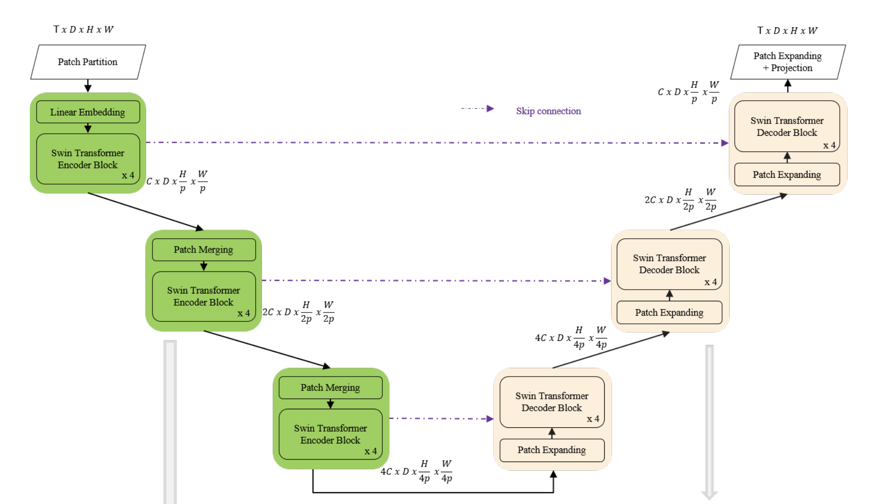
Spatial downsampling is applied to reduce the embedding space. We used a fully connected layer to scale up the dimension of the incoming data.
The proposed network is tested on the Weather4Cast2021 weather forecasting challenge data, which requires the prediction of 8 hours ahead future frames (4 per hour) from an hour weather product sequence.
This paper used 3D patch embedding, 3D shifted window multi-head self attention as well as patch merging. This paper has 2d variables as channel dimension is not patchified. In my case we'll need to create 4D patch embedding as also height layer has to be partitioned.
Multi-scaled stacked ViT
Development of an efficient ViT:
- Adds a layer normalization after the patch embedding operation;
- Global and Local token differentiation;
- Self-attention mechanism is replaced with efficient multi-scaled self-attention mechanism;
- Positional embedding 1-D is replaced with 2-D positional embedding or absolute positional bias.
Multi-scaled self-attention mechanism
Uses a local attention plus global memory approach. Define the n_g global tokens that are allowed to attend to to all tokens, and the n_l local tokens that are allowed to attend to the tokens in their local 2D window area and only the global tokens.
Relative positional bias: add a bias matrix to each head when capturing the attention score (makes the transfomer translation invariant).
Theoretical complexity: n_g and n_l are global and local token numbers, the memory complexity is \( O( n_g(n_g + n_l) + n_l w^2 ) \).
Comparisons
Linformer: projects \( n_l \times d \) dimensional keys and values to \( K \times d \) with an additional linear projection layer, where \( K << n_l \). The memory complexity in this case is \( O( K n_l ) \) where K is a constant, usually set to 256.
Performer: uses random kernels to approximate the softmax in MSA.
How to compare? It depends a lot on the trade-offs. More aggressive spatial resolution makes accuracy worst, but performance is much better (or memory cost manageable).
Why is longformer better? Conv-like sparsity gives better inductive bias for ViTs. Or, the Longformer keeps keys and values at high resolution.
Linear Transformers
Introduction
How to rout information in a sequence of tokens? -> We use query + key matrices
- Query: what we are looking for (what info we want to extract)
- Key: what type of info the node contains (what info we have)
Inner product is used to rout (similarity between query and key). This is called soft-routing as it is a weighted average of all the keys (where inner product is larger).
Complexity is \( O(n^2) \), where n is the number of tokens (sequence length), embedding size is d.
\( Q \times K = n \times n \) -> where multi-head attention doesn't help, but the n matrix could be simplified into n/heads matrix.
Ex. 4 heads -> 512 / 4 = 128
We can approximate Q into a low rank matrix, and complexity would be reduced to \( O(n) \).
Linear Transformer
\( \text{Attention} = \text{softmax}(\frac{QK^T}{\sqrt{d_k}})V \)
If the term inside the softmax is low rank, then we can reduce computation.
Eigenvalues of Q and K can be used to determine if matrix needs to be high or low rank. Results show that most of the times 128 is enough.
How to reduce dimensionality? We can use a random projection P before the self-attention layer.
\( \text{Attention} = \text{softmax}(\frac{Q(EK)^T}{\sqrt{d_k}})FV \)
So we introduce the E and F matrices (fixed, not learned). The term inside the softmax becomes nxk, while FV is kxn. The shapes so are correct for matmult.
Results
With large sequence lengths, the linear transformer keeps inference times constant, as it doesn't depend on the sequence length n but also on k. Complexity is reduced from \( O(n^2) \) to \( O(nk) \).
How to choose k?
\( k = \frac{5\log(n)}{c} \)
So it depends on n still? Complexity is \( O(n\log(n)) \) now.
However we can make it linear:
\( k = min { \theta(9d \log(d)), 5\theta(\log(n)) } \)
In the first case it is linear in d, in the second case it is linear in n. We can choose the minimum of the two. So it's enough to downproject the matrix to a dimension of about d.
Linear Transformers as FWP
Introduction
The concept of fast weight programmers (FWP) is introduced in this paper.
The idea is to use a slow network to program by gradient descent the weights of a fast network. FWP learn to pmanipulate the content of a finite memory and dynamically interact with it.
Linear transformers have constant memory size and time complexity linear which depends on the sequence length. The time complexity is reduced thanks to the linearization of the self-attention layer and softmax operation.
Linear Transformers as FWP
In normal neural networks, the weights are fixed and the input is manipulated, while the activation is input dependant and can change at inference time. The idea of FWP is also have the weights variable and input dependent (synaptic modulation).
- Context-dependent -> slow weights
- Context-independent -> fast weights
The process revolves around a slow network which is trained to program the weights of the fast network. This makes the fast weights dependent on the spatio-temporal context of the input stream.
Which instructions to use? Outer product:
\( a^{(i)}, b^{(i)} = W_ax^{(i)}, W_bx^{(i)} \) \( W^{(i)} = \sigma (W^{(i-1) + a^{(i)} \oplus b^{(i)}}) \) \( y^{(i)} = W^{(i)} x^{(i)} \)
The outer product is \( \oplus \), \sigma is the activation function, W_a and W_b are the trainable slow weights, while W is the fast weight matrix.
Linearizing self-attention
Instead of removing the softmax, prior works have introduced techniques for linearizing the softmax. This improves the computational efficiency of the self-attention layer for long sequences.
An important term is the softmax kernel \( \kappa(k, q) = exp(k \dot q) \), which in linear self-attention is approximated by another kernel \( \kappa'(k, q) = \phi(k)^T \phi(q) \).
Since the embedding space for keys is limited, there is only room for d orthogonal vectors. If the length of the sequence is larger than d, th model might be in a overcapacity regime. In this case the model should dynamically interact with the memory content and determine which association to remember and which one to forget. On the other hand, the standard transformer stores associations as immutable pairs, increasing its memory requirements.
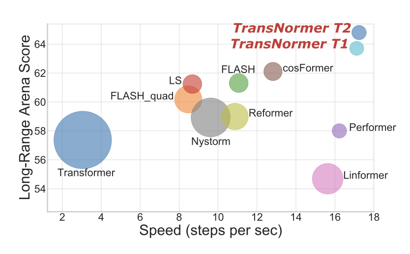
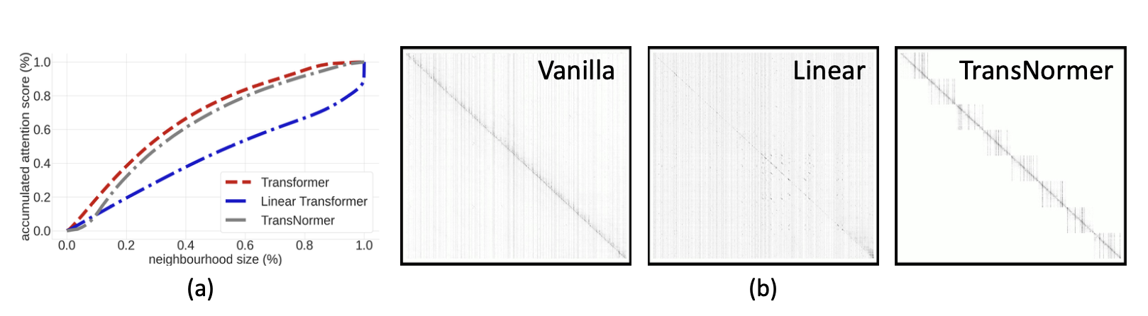
The Devil in Linear Transformers
Summary
Kernel based linear transformer have two main problems:
- Unbounded gradients: which negatively affect convergence (the problem comes from the scaling of the attention matrix);
- Attention dilution: which trivially distributes attention scores along large sequences.
The authors propose a solution to both problems by introducing a new model, the Transnormer. The idea is to used vanilla attention, which is more accurate and causes less dilution, in conjunction with linear attention, which is more efficient and scalable.
- Diagonal attentin is used for the early stages of the network, to address dilution;
- Norm attention is used in later stages, to stabilize training gradients.
Can we just remove scaling from linear attention? No, because it would cause a drop in accuracy (ppl). The cause is that the attention map becomes unbounded in the forward pass. We want to bound attention map in forward, as well as gradients in backward pass.
Attention without scaling can be calculated as follows:
\( O = Q(K^TV) \) \( O_{norm} = X_{norm}(Q(K^TV)) \)
where \( X_{norm} \) is a normalization layer.
Diagonal attention on the other hand is created by leveraging a non-overlapping blocks strategy for the attention distribution. This reduces time complexity as attention is calculated inside each block.
Complexity is given by:
\( O(nwd) \)
where \( n \) is the sequence length, \( w \) is the block size, and \( d \) is the feature dimension.
This concludes that these models require global attention in later stages, while local attention is sufficient in early stages.
Do Vision transformers share the same issues?
Performer
Estimates regular self attention with provable accuracy in linear space and time complexity. Uses Fast Attention Via Orthogonal Random Features (FAVOR+) to approximate the softmax attention mechanism. (Scalable kernel method)
Normally attention is calculated as follows:
\( Attn(Q, K, V) = D^{-1}AV \)
Where \( A = exp(QK^T / \sqrt{d}) \) and \( D = diag(A1_L) \) (1 is a vector of ones)
The Performer approximates the softmax attention mechanism by using orthogonal random features. The attention mechanism is approximated as follows:
\( Attn(Q, K, V) = \hat{D}^{-1}\hat{A}V \)
Where \( \hat{A} = tril(A) \) and \( \hat{D} = diag(\hat{A}1_L) \), and tril() returns the lower triangular part of the argument matrix including the diagonal.
The attention matrix can be calculated in \( O(Ld^2 log(d)) \) where \( L \) is the sequence length and \( d \) is the hidden dimension. While normally the attention matrix is calculated in \( O(Ld^2 log(L) ) \) time.
SRFormer
Introduces permuted self attention, which can be added to the normal window self-attention.
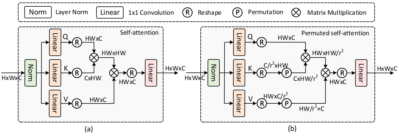
How do we increase the attention window without increasing the complexity?
Given a feature map X and a token reduction factor r, we first split X into non overlapping square windows with side length S. The result is then passed through 3 linear layers to get Q, K and V.
Compress K and V size to \( \frac{NS^2}{r^2C} \), then permute the spatial tokens in K and V to the channel dimension, obtaining K_p and V_p.
The self-attention window size becomes \( \frac{S}{r} \times \frac{S}{r} \), but C is unchanged.
The performance gain is obtained when downscaling the spatial dimension, as the complexity of the attention mechanism is reduced.
Test time training (TTT)
- Transformers: O(N^2) complexity due to self-attention.
- Mamba and advanced RNNs: O(N) complexity, but latent space is fixed, still subject to catastrophic forgetting
TTT methods
New class of sequence modelling layers where the hidden state is a model, and the update rule is a step of self-supervised learning. The process is updating the hidden state even during the test time.
Self attention has hidden state growing linearly with the sequence length (cost is per token), while TTT has a fixed size hidden state.
TTT compresses the historical context into a hiddden state St, making the context an unlabelled dataset.
Test Time Training ++
Can TTT always mitigate distributional shift? This paper shows an improved version of TTT
TTT adapts neural networks to new data distributions at test time on unlabeled samples, using two tasks:
- Main task (classification)
- Auxiliary task (SSL reinforcement)
When does it fail?
- When the auxiliary task is not informative
- When the auxiliary task overfits --> main task may worsen
Solution: Online feature alignment (domain adaptation with divergence measure). After training we have offline feature summarization (mean and std calculation), channel wise batch norm using stats just calculated, then test time regularization minimizing the distance between test and train samples.
- Online dynamic queue
TTT-A: alignment of features (first + second order statistics) TTT-C: contrastive learning addition (SSL on target domain)
TTT++: TTT-A + TTT-C
Limits: feature summarization + resnet backbone
Universal Transformers
RNNs: slow in training
Feedforward and conv architectures have achived better performance in many tasks, but transformers fail in generalizing for simple tasks.
Universal Transformers: parallel in time, self-attentive RNN, combines recurrent nature + simple parallelization of transformers. It can also be tuting complete if given enough data (SOTA performance on many tasks).
UT refines a series of vector representations at each position of the sequence in parallel. It combines info with self-attention + recursive transition function across all time steps.
![]()
How is efficiency?
With enough computation, UT is computationally universal.
The Rise of Data-Driven Weather Forecasting
Summary
Comparison between AI based forecasts and NWP forecasts in operational-like context. The rise was due to the availability of large datasets and the development of new models. Examples include ERA5 reanalysis (28km resolution, 0.25 degs, 1979-2019). The use of this dataset however renders the resolution of the models to be lower compared to IFS, which is 9km.
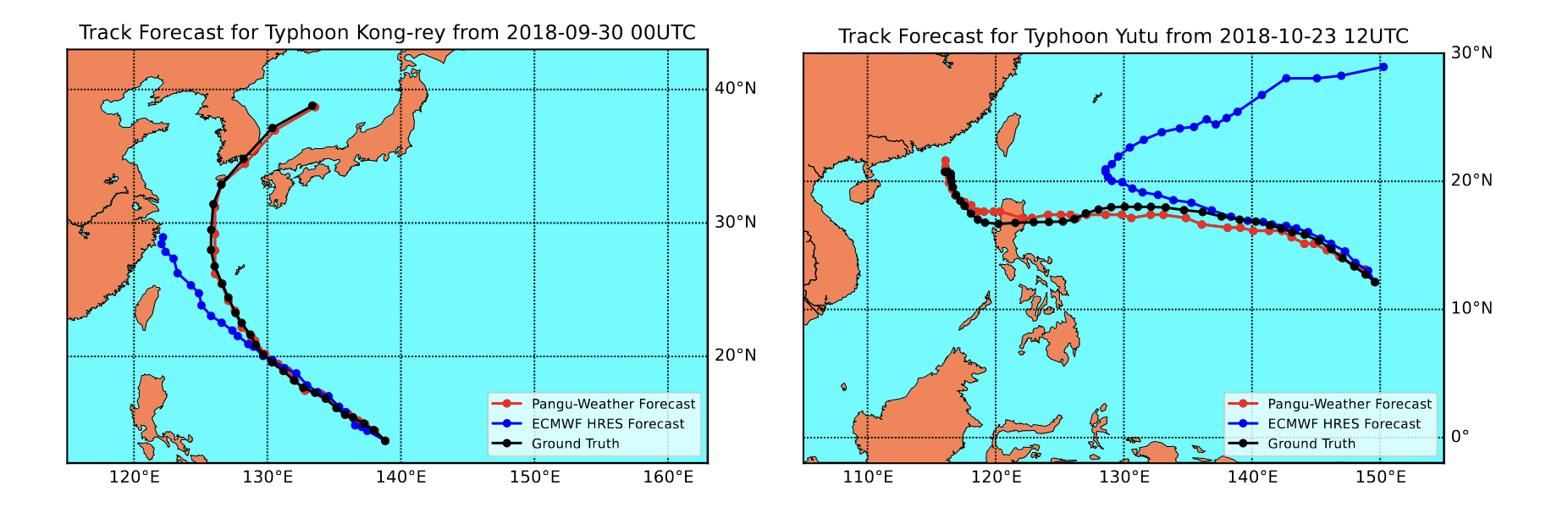
Comparison Pangu-IFS:
- Statistical consistency of the model: IFS is better than PGW, which is far from perfect reliability. Can the model predicti extreme events with the same probability as the observations? (or is it just blurring?) Used example is the one of tropical cyclones.
- Forecast error prediction: general agreement between PGW and IFS in daily mean error.
ClimaX
ClimaX is a foundation model designed to be pre-trained on heterogeneous data sources and then fine-tuned to solve various downstream weather and climate problems.
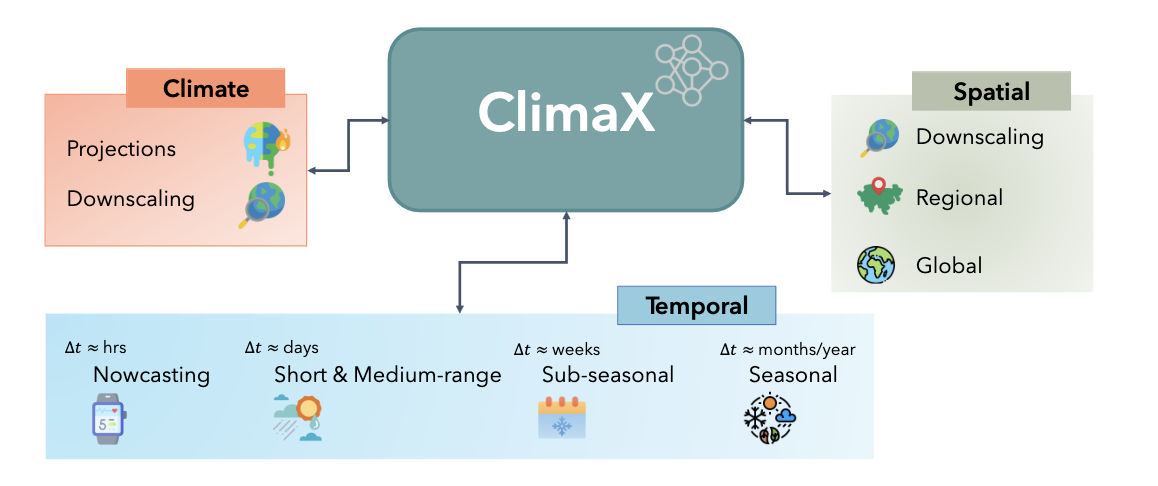
The set of climate and weather variables is extremely broad, and predictions may be required for regional or even spatially incomplete data, even at different resolutions. Current CNN-based architectures are not applicable in these scenarios, as they require the input to be perfectly gridded, contain a fixed set of variables, and have a fixed spatial resolution. resolution. Transformer-based architectures, on the other hand, offer much greater flexibility by treating the image-like data as a set of tokens. As a consequence, the backbone architecture chosen is a Vision Transformer to provide greater flexibility.
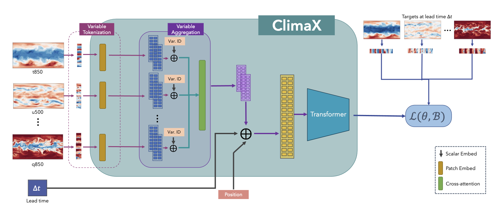
Two significant changes to this model were implemented. The first change involved variable tokenization, which includes separating each variable into its own channel and tokenizing the input into a sequence of patches. The second change was variable aggregation, introduced to speed up computation by reducing the dimensionality of the input data and to aid in distinguishing between different variables, thereby enhancing attention-based training. After combining variables, the vision transformer block can produce output tokens that are then processed through a linear prediction head to recreate the original image. During the pre-training phase, a latitude-weighted reconstruction error is used to keep into account the location of the current patch. For fine-tuning, the ClimaX modules can be frozen, allowing for training only on the intended part of the architecture. In fact, often only the final prediction head and variable coding modules need retraining. This model has undergone testing for several downstream tasks, including global and regional forecasting and prediction for unseen climate tasks.
PanguWeather
Pangu Weather is a transformer architecture trained on three dimensional weather variables, as opposed to Climax, where all data was two dimensional. The lead time is also handled differently, with the model being trained to predict the weather at a certain time in the future, as opposed to the approach taken in the ClimaX work, where the lead time is passed as a parameter during the training phase.
The former approach is more similar to the one used in this project, where the simplicity of the dataset allows for a more straightforward implementation of the lead time, sacrificing some flexibility in the process. Finally, the Pangu weather model features some advanced techniques which separate it from all other competitors, namely the use of two different resolutions for the encoding of each variable, allowing the model to capture both large scale and small scale features, and use the attention mechanism to focus on different parts of the input data at the same time.
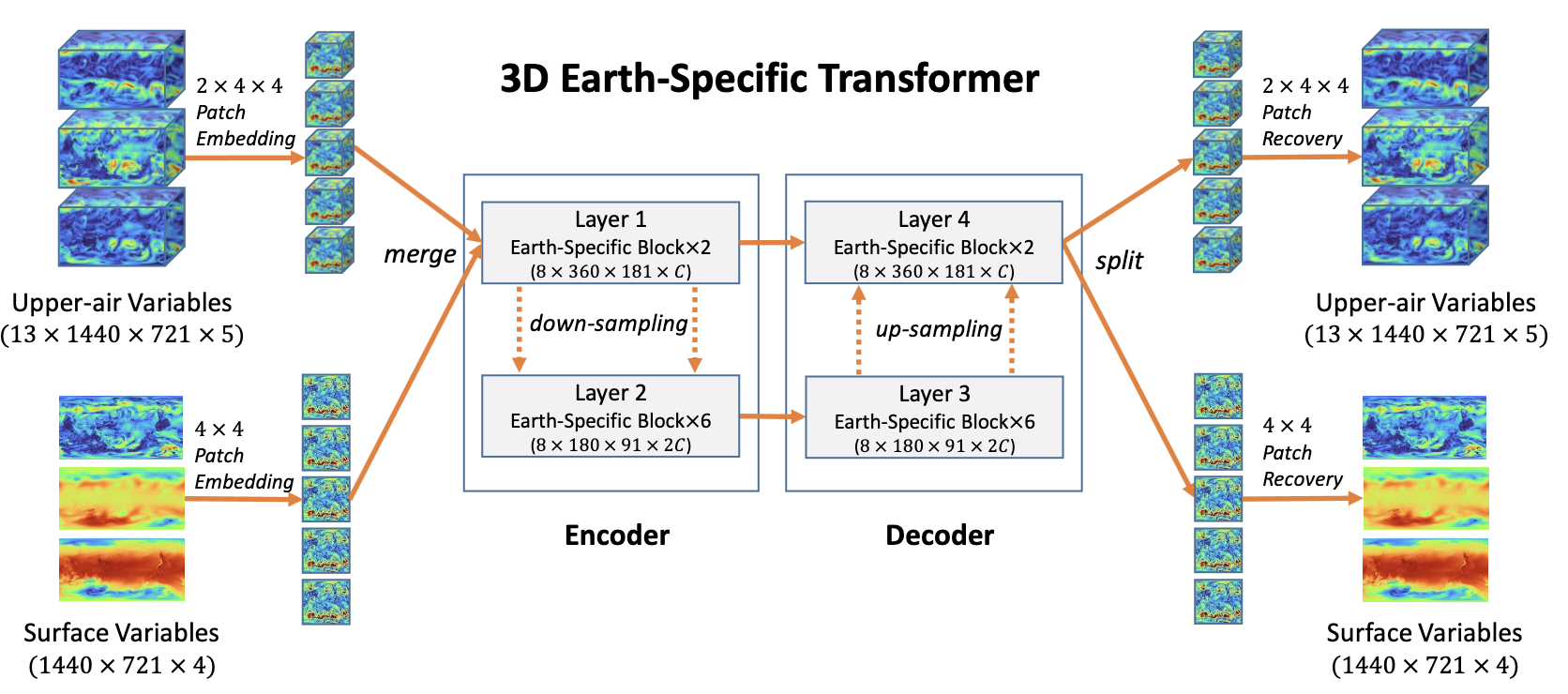
To achieve these two resolution, an encoder-decoder approach is used, where the encoder is tasked with the downscaling of input variables, and the decoder is tasked with the upscaling of the output. All transformer blocks are then applied to the output of the encoder, taking as input both the low and high resolution information.
MetNet 3
- Temporal resolution: 2 minutes
- Spatial resolution: 1 km
The network is a U-Net in conjunction with a MaxVit architecture
- Topographical embedding: automatically embeds time-indipendent variables (4km tokens) for 20 parameters
- U-Net: based on a fully convolutional neural network whose architecture was modified and extended to work with fewer training images and to yield more precise segmentation
- MaxVit: hybrid (CNN + ViT) image classification models.
Uses parameter oriented training for lead time (0 - 24 hours). Masks out with 25% probability a block of data.
FuXi
FuXi is an auto-regressive model for weather forecasting. The model is based on the U-transformer architecture, and is able to recurrently produce a prediction for the next timestep, given the previous predictions.

To generate a 15 days forecast, it is estimated it takes the model around 60 iterations, with a lead time of 6 hours. The loss utilized is multi-step, meaning it takes into account several timesteps at once, minimizing the error for each of them. This is in contrast with the approach taken in this project, where the loss is computed for each timestep individually. The U-transformer takes as input around 70 variables, for the current timestep, as well as the the preceding frame. All the variables used for this model are however restricted to two dimensions, ignoring any height layer. This architecture is a variation of the vanilla transformer model, and as opposed to the latter, before passing the encoded information to the self attention blocks, it downscales partially the input.
FourcastNet
FourcastNet is an architecture based on the Adaptive Fourier Neural Operator, which is a neural network model designed for high-resolution inputs, fused with a vision transformer backbone. The Fourier Neural Operator is a neural network architecture that uses a Fourier basis to represent the input data, allowing for the efficient computation of convolutions in the Fourier domain.

The use of this module allows to have a very small footprint in GPU memory, which is crucial for the training of large models. For instance, the base model used is around 10Gb in size, while analogue models with similar number of parameters have a size of around eight times as large.
GraphCast
Graphcast is a graph neural network architecture with an encoder-decoder configuration. The graph neural network is used to encode unstructured input data into a graph representation. As opposed to, for instance, convolutional layers where neighbouring information is encoded in a structured grid, graph layers use message passing between nodes to capture the relationships between different parts of the input data. This allows for the encoding of different kind of information, not necessarily restricted to a grid configuration.

One important hyperparamter to be set in this kind of architectures is the number of hops the messages containing neighbouring information are allowed to travel. This is crucial for the model to learn from the correct amount of knowledge, and allows for reducing the computational complexity of the model, as the number of hops is directly related to the time required for the model to train.

PrithViWxC (NASA FM)
2.3B Params, 160 variables from MERRA-2 (New ERA5)
Encoder-decoder architecture (MAE) ~50% masking operator probability
Tested on:
- Autoregressive rollout forecasting
- Gravity waveflux parameterization: small scale perturbations generated around thunderstorms
- Extreme event estimation
Max-ViT + HieraViT approaches:
- Axial Attention (with convolutional layers)
- Add convolutions at finetune to improve performance
- Local + Global attention Uses Flash Attention and FSDP
Validation with:
- Zero shot reconstruction
- Hurricane tracking
- Downscaling
MERRA2 dataset: cubed sphere grid, uniform grid spacing for each lat/lon (it minimizes grid spacing irregularities).
Climatology: instead of predicting delta from current time, we predict the delta from historical climate C_t. It is calculated from merra with 61 days of rolling average (it is computed across space and time).
Sigma^2_c = Sigma^2_c (x_t - C_t)
Normalization is also applied (10^-4 < sigma < 10^4, and 10^-7 < sigma_c < 10^7)
Scaling and training
Pretraining with 2 phases:
-
- 5% drop path rate, 50% masking operator probability, alternates global and local attention masking. Uses random forecast lead time (0, 6, 12, 24 hours). Train on 64 A100 GPUs, Batch size = 1, ~100000 gradient steps.
-
- 4 autoregressive steps with 80GB A100 GPUs. Use bfloat16 precision to shrink activation buffer sizes (and encoder / decoder size) while i/o remains f32
-
- 2 phases in pretraining with different masking ratios and params
Validation
- Masked reconstruction from zero-shot images
- Hurricane forecasting and tracking
Downstream applications:
- Downscaling for 2m precision + climatelearn benchmark
- Finetune for cordex downscaling
- Zero-shot masked reconstruction --> excels at short lead time prediction from minimal data.
Oak Ridge base FM for Earth System Predictability
113B parameters with hybrid tensor data orthogonal parallelism technique (Hybrid STOP)
Uses unique math property of matrix chain multiplpication distributes model parameters in alternating row/columns shards. It combines tensor parallelism + FSDP. Better scalablity, avoids peak memory usage, keeps parameters shared through memory
y = xAB
It gathers partially and not globally, which makes the process faster on memory.
Uses 684 PetaFLOPS to 1.6 ExaFLOPS throughput across 49152 GPUs.
91 climate variables from 10 CMIP datasets, 1.2M data points.
Optimizations:
- Architecture optimization: problematic convergence with large attention logits (adds layer normalization before the self attention)
- Hierarchical parallelism: add also DDP on top of H-STOP (this speeds up training)
- Activation checkpoints: trade compute for memory savings in LLMs
- Mixed Precision: use bfloat16 to make large computations easier
- Layer wrapping: iterative FSDP sharding and prefetch
ClimateLearn
Summary
Aims at aiding climate forecasting, downscaling and projections.
It is a pytorch integrated dataset, composed mainly of CMIP6, ERA5 and PRISM data.
-
Forecasting: close to medium range weather and climate prediction
-
Downscaling: Due to large grid sizes, large cells are often used for reducing size of data. However, this leads to loss of information, and to a lower resolution predictions. Downscaling aims at correcting bias amd map results to higher resolution.
\( C \times W \times H \leftarrow C' \times W \times H \) where \( H < H' \) and \( W < W' \)
-
Projections: Obtaining long range predictions under different conditions (ex. greenhouse gasses emission or atmosphere composition).
The library also includes several baselines, pipelines for end-to-end training and evaluation, and a set of metrics.
ClimateBench
Summary
The aim is to simulate shared socio-economic pathways.
It is a benchmarking framework from CMIP, AerChemMIP, ScenarioMIP, and Detection-AttributionMIP. It also contains several ML models and full complexity Earth System Models (ESMs).
Mostly used for long term projections.
Also includes piControl (pre-industrial control, 500 years of points) and historical (historical forcing) simulations, which can be used for contrastive learning to reduce the amount of samples required by ML models, as for projections not enough data is available for deep learning training.
A possible challenge is applying ML and statistical learning to high-dimensional data. To this end Linear Transformers could be used.
WeatherBench
New benchmark to evaluate data-driven weather forecasting models (deep learning). The benchmark task is to predict pressure and temperature 3-5 days in advance.
The dataset used is ERA5 (40 years), regridded to lower resolution (bilinear interpolation) and usinfg 13 height levels:
- 5.625 degrees (32x64 grid)
- 2.8125 degrees (64x128 grid)
- 1.40625 degrees (128x256 grid)
Evaluation is executed on 2017 and 2018.
RMSE is used as the evaluation metric, also latitude-weighted RMSE.
Baselines:
- Operational NWP models (ECMWF, IFS)
- Linear Regression
- Simple CNN
Weather Challenges
- 3D atmosphere (CNNs might not work if used as channels)
- Limited train data (samples are correlated in time)
- Data is heavy to store in GPU memory
Extreme situations forecast: used as validation, to make sure the model is not just blurring (averaging) the predictions.
Key Features of WeatherBench
- Scientific Impact: of computing these models
- Challenge for data science
- Clear metrics for the climate domain
- Quickstart for users
- Reproducibility + communication between researchers
IPCC Working Group 1
The Current State of the Climate
It is unequivocal that human influence has warmed the atmosphere, ocean and land. Widespread and rapid changes in the atmosphere, ocean, cryosphere and biosphere have occurred.
Global mean sea level increased by 0.20 [0.15 to 0.25] m between 1901 and 2018. The average rate of sea level rise was 1.3 [0.6 to 2.1] mm yr–1 between 1901 and 1971, increasing to 1.9 [0.8 to 2.9] mm yr–1 between 1971 and 2006, and further increasing to 3.7 [3.2 to 4.2] mm yr–1 between 2006 and 2018 (high confidence). Human influence was very likely the main driver of these increases since at least 1971.
Human-induced climate change is already affecting many weather and climate extremes in every region across the globe.
Improved knowledge of climate processes, paleoclimate evidence and the response of the climate system to increasing radiative forcing gives a best estimate of equilibrium climate sensitivity of 3°C.
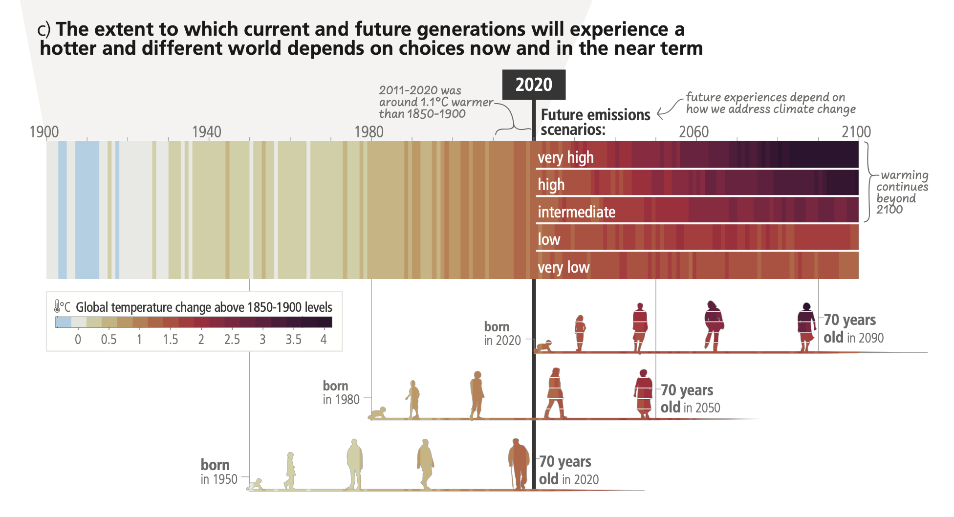
Possible Climate Futures
Global surface temperature will continue to increase until at least mid-century under all emissions scenarios considered. Global warming of 1.5°C and 2°C will be exceeded during the 21st century unless deep reductions in CO2 and other greenhouse gas emissions occur in the coming decades.
Many changes in the climate system become larger in direct relation to increasing global warming. They include increases in the frequency and intensity of hot extremes, marine heatwaves, heavy precipitation, and, in some regions, agricultural and ecological droughts; an increase in the proportion of intense tropical cyclones; and reductions in Arctic sea ice, snow cover and permafrost.
It is virtually certain that the land surface will continue to warm more than the ocean surface. It is virtually certain that the Arctic will continue to warm more than global surface temperature, with high confidence above two times the rate of global warming.
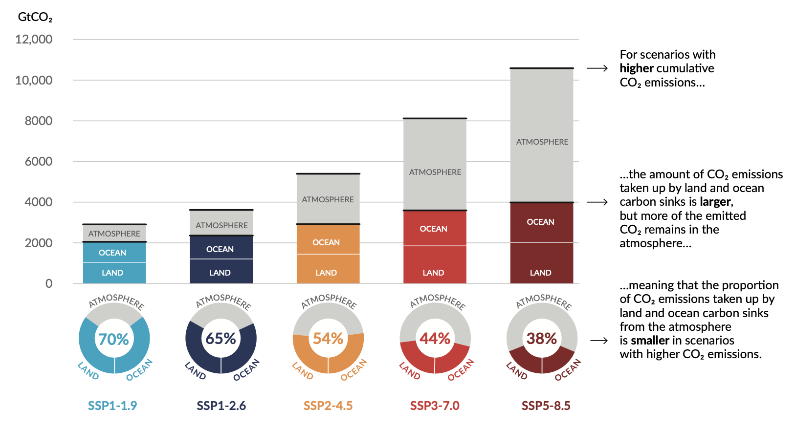
Continued global warming is projected to further intensify the global water cycle, including its variability, global monsoon precipitation and the severity of wet and dry events. Also, under scenarios with increasing CO2 emissions, the ocean and land carbon sinks are projected to be less effective at slowing the accumulation of CO2 in the atmosphere.
Many changes due to past and future greenhouse gas emissions are irreversible for centuries to millennia, especially changes in the ocean, ice sheets and global sea level.
IPCC Working Group 2
Observed and Projected Impacts and Risks
Human-induced climate change, including more frequent and intense extreme events, has caused widespread adverse impacts and related losses and damages to nature and people, beyond natural climate variability. Vulnerability of ecosystems and people to climate change differs substantially among and within regions driven by patterns of intersecting socioeconomic development, unsustainable ocean and land use, inequity, marginalization, historical and ongoing patterns of inequity such as colonialism, and governance.
Current unsustainable development patterns are increasing exposure of ecosystems and people to climate hazards.
Risks in the near term (2021–2040)
Global warming, reaching 1.5°C in the near-term, would cause unavoidable increases in multiple climate hazards and present multiple risks to ecosystems and humans.
Mid to Long-term Risks (2041–2100)
Beyond 2040 and depending on the level of global warming, climate change will lead to numerous risks to natural and human systems. The magnitude and rate of climate change and associated risks depend strongly on near-term mitigation and adaptation actions, and projected adverse impacts and related losses and damages escalate with every increment of global warming
IPCC Working Group 3
Recent Developments and Current Trends
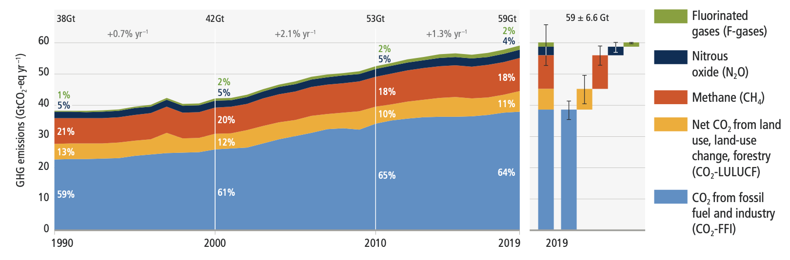
Total net anthropogenic GHG emissions6 have continued to rise during the period 2010–2019, as have cumulative net CO2 emissions since 1850. Regional contributions to global GHG emissions continue to differ widely. Variations in regional, and national per capita emissions partly reflect different development stages, but they also vary widely at similar income levels. The 10% of households with the highest per capita emissions contribute a disproportionately large share of global household GHG emissions. At least 18 countries have sustained GHG emission reductions for longer than 10 years.
Globally, the 10% of households with the highest per capita emissions contribute 34–45% of global consumption-based household GHG emissions,21 while the middle 40% contribute 40–53%, and the bottom 50% contribute 13–15%.
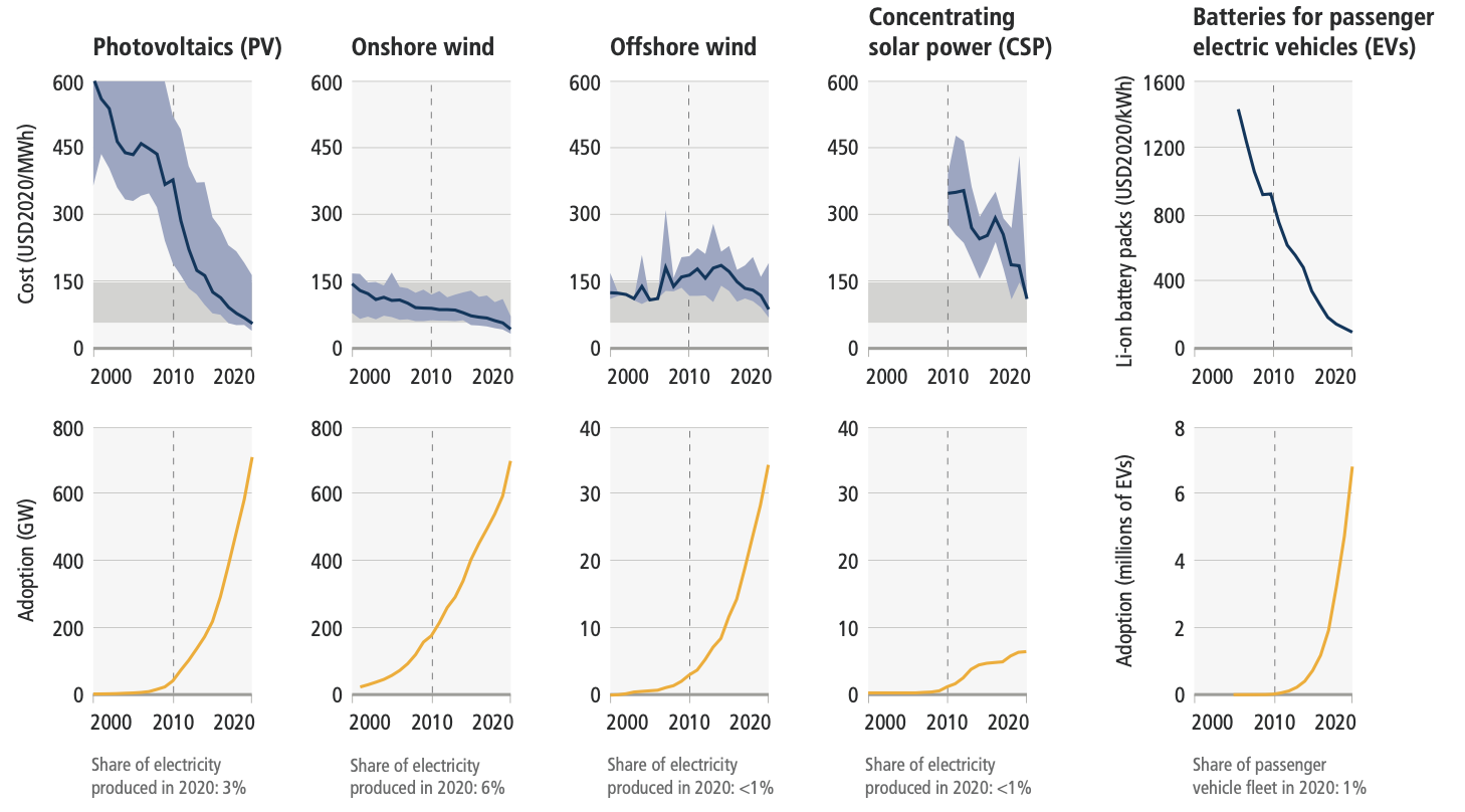
The unit costs of several low-emission technologies have fallen continuously since 2010. Innovation policy packages have enabled these cost reductions and supported global adoption.
There has been a consistent expansion of policies and laws addressing mitigation since AR5. This has led to the avoidance of emissions that would otherwise have occurred and increased investment in low-GHG technologies and infrastructure. Policy coverage of emissions is uneven across sectors.
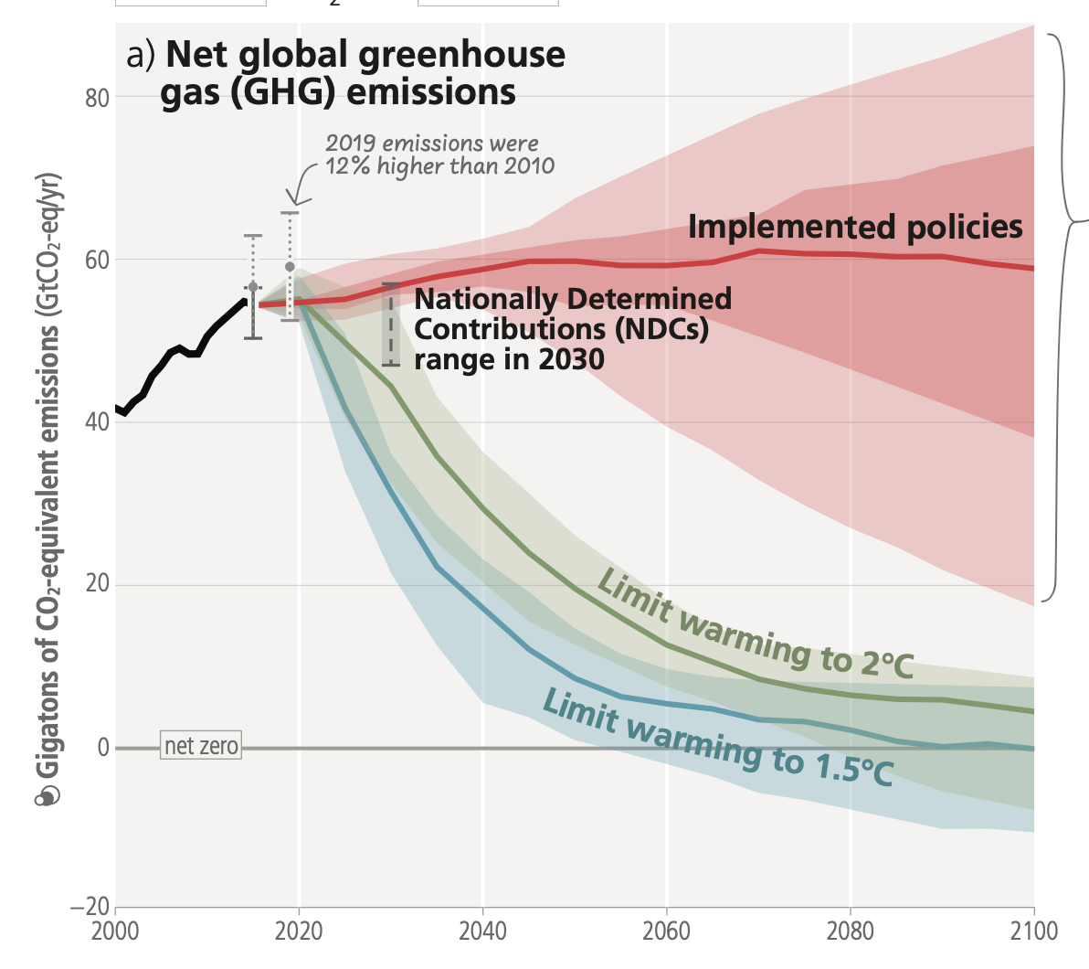
Global GHG emissions in 2030 associated with the implementation of Nationally Determined Contributions (NDCs) announced prior to COP2623 would make it likely that warming will exceed 1.5°C during the 21st century.24 Likely limiting warming to below 2°C would then rely on a rapid acceleration of mitigation efforts after 2030.
System Transformations to Limit Global Warming
Global GHG emissions are projected to peak between 2020 and at the latest before 2025 in global modelled pathways that limit warming to 1.5°C (>50%) with no or limited overshoot and in those that limit warming to 2°C (>67%) and assume immediate action. Without a strengthening of policies beyond those that are implemented by the end of 2020, GHG emissions are projected to rise beyond 2025, leading to a median global warming of 3.2°C by 2100.
All global modelled pathways that limit warming to 1.5°C (>50%) with no or limited overshoot, and those that limit warming to 2°C (>67%), involve rapid and deep and in most cases immediate GHG emission reductions in all sectors.
This would involve very low or zero-carbon energy sources, such as renewables or fossil fuels with CCS, demand side measures and improving efficiency, reducing non-CO2 emissions, and deploying carbon dioxide removal (CDR) methods to counterbalance residual GHG emissions.
Reducing GHG emissions across the full energy sector requires major transitions, including a substantial reduction in overall fossil fuel use, the deployment of low-emission energy sources, switching to alternative energy carriers, and energy efficiency and conservation.
Net zero CO2 emissions from the industrial sector are challenging but possible. Reducing industry emissions will entail coordinated action throughout value chains to promote all mitigation options, including demand management, energy and materials efficiency, circular material flows, as well as abatement technologies and transformational changes in production processes.
Urban areas can create opportunities to increase resource efficiency and significantly reduce GHG emissions through the systemic transition of infrastructure and urban form through low-emission development pathways towards net-zero emissions.
In modelled global scenarios, existing buildings, if retrofitted, and buildings yet to be built, are projected to approach net zero GHG emissions in 2050 if policy packages, which combine ambitious sufficiency, efficiency, and renewable energy measures, are effectively implemented and barriers to decarbonisation are removed.
The deployment of carbon dioxide removal (CDR) to counterbalance hard-to-abate residual emissions is unavoidable if net zero CO2 or GHG emissions are to be achieved. The scale and timing of deployment will depend on the trajectories of gross emission reductions in different sectors.
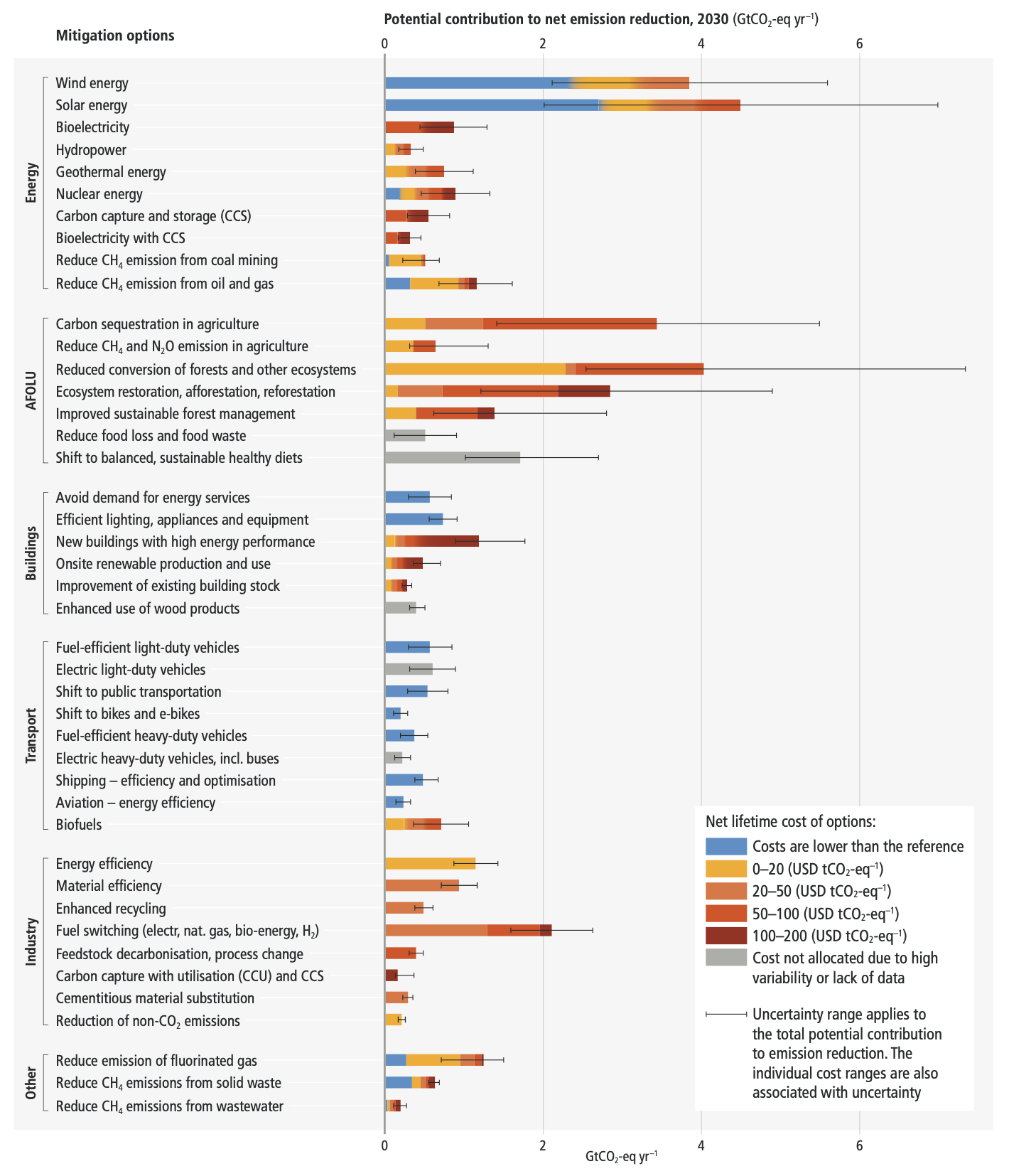
Mitigation options costing USD100 tCO2-eq–1 or less could reduce global GHG emissions by at least half the 2019 level by 2030.
IPCC Assessment Report 6
Introduction
Assessment Report (AR6) summarises the state of knowledge of climate change, its widespread impacts and risks, and climate change mitigation and adaptation. It integrates the main findings of the Sixth Assessment Report (AR6) based on contributions from the three Working Groups
Current Status and Trends
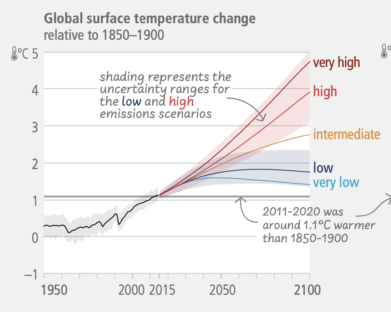
Human activities, principally through emissions of greenhouse gases, have unequivocally caused global warming, with global surface temperature reaching 1.1°C above 1850-1900 in 2011-2020. The likely range of total human-caused global surface temperature increase from 1850–1900 to 2010–20197 is 0.8°C to 1.3°C, with a best estimate of 1.07°C.
Widespread and rapid changes in the atmosphere, ocean, cryosphere and biosphere have occurred. Human-caused climate change is already affecting many weather and climate extremes in every region across the globe. This has led to widespread adverse impacts and related losses and damages to nature and people. Vulnerable communities who have historically contributed the least to current climate change are disproportionately affected.
Approximately 3.3 to 3.6 billion people live in contexts that are highly vulnerable to climate change. Human and ecosystem vulnerability are interdependent. Regions and people with considerable development constraints have high vulnerability to climatic hazards.
Impacts on some ecosystems are approaching irreversibility such as the impacts of hydrological changes resulting from the retreat of glaciers, or the changes in some mountain and Arctic ecosystems driven by permafrost thaw.
Climate change has reduced food security and affected water security, hindering efforts to meet Sustainable Development Goals. In all regions increases in extreme heat events have resulted in human mortality and morbidity. The occurrence of climate-related food-borne and water-borne diseases and the incidence of vector-borne diseases have increased. In assessed regions, some mental health challenges are associated with increasing temperatures.
Adaptation planning and implementation has progressed across all sectors and regions, with documented benefits and varying effectiveness. Despite progress, adaptation gaps exist, and will continue to grow at current rates of implementation.
Growing public and political awareness of climate impacts and risks has resulted in at least 170 countries and many cities including adaptation in their climate policies and planning processes. Maladaptation especially affects marginalised and vulnerable groups adversely. Key barriers to adaptation are limited resources, lack of private sector and citizen engagement, insufficient mobilization of finance (including for research), low climate literacy, lack of political commitment, limited research and/or slow and low uptake of adaptation science, and low sense of urgency.
Policies and laws addressing mitigation have consistently expanded since AR5. Global GHG emissions in 2030 implied by nationally determined contributions (NDCs) announced by October 2021 make it likely that warming will exceed 1.5°C during the 21st century and make it harder to limit warming below 2°C. There are gaps between projected emissions from implemented policies and those from NDCs and finance flows fall short of the levels needed to meet climate goals across all sectors and regions.
From 2010 to 2019 there have been sustained decreases in the unit costs of solar energy (85%), wind energy (55%), and lithium-ion batteries (85%), and large increases in their deployment.
Policies implemented by the end of 2020 are projected to result in higher global GHG emissions in 2030 than emissions implied by NDCs, indicating an ‘implementation gap’.
Future Climate Change, Risks, and Long-Term Responses
Continued greenhouse gas emissions will lead to increasing global warming, with the best estimate of reaching 1.5°C in the near term in considered scenarios and modelled pathways. Every increment of global warming will intensify multiple and concurrent hazards.
Global warming will continue to increase in the near term (2021–2040) mainly due to increased cumulative CO2 emissions in nearly all considered scenarios and modelled pathways. In the near term, global warming is more likely than not to reach 1.5°C even under the very low GHG emission scenario and likely or very likely to exceed 1.5°C under higher emissions scenarios.
With further warming, every region is projected to increasingly experience concurrent and multiple changes in climatic impact-drivers. Compound heatwaves and droughts are projected to become more frequent, including concurrent events across multiple locations. Projected regional changes include intensification of tropical cyclones and/or extratropical storms, and increases in aridity and fire weather.
With every increment of global warming, regional changes in mean climate and extremes become more widespread and pronounced. Risks and projected adverse impacts and related losses and damages from climate change escalate with every increment of global warming. The level of risk will also depend on trends in vulnerability and exposure of humans and ecosystems. Future exposure to climatic hazards is increasing globally due to socio-economic development trends including migration, growing inequality and urbanisation.
Some future changes are unavoidable and/or irreversible but can be limited by deep, rapid, and sustained global greenhouse gas emissions reduction. The likelihood of abrupt and/or irreversible changes increases with higher global warming levels. Deep, rapid, and sustained GHG emissions reductions would limit further sea level rise acceleration and projected long-term sea level rise commitment.
As warming levels increase, so do the risks of species extinction or irreversible loss of biodiversity in ecosystems including forests, coral reefs, and in Arctic regions.
Adaptation options that are feasible and effective today will become constrained and less effective with increasing global warming. With increasing global warming, losses and damages will increase and additional human and natural systems will reach adaptation limits.
Limiting human-caused global warming requires net zero CO2 emissions. Cumulative carbon emissions until the time of reaching net zero CO2 emissions and the level of greenhouse gas emission reductions this decade largely determine whether warming can be limited to 1.5°C or 2°C. All global modelled pathways that limit warming to 1.5°C (>50%) with no or limited overshoot, and those that limit warming to 2°C (>67%), involve rapid and deep and, in most cases, immediate greenhouse gas emissions reductions in all sectors this decade.
If warming exceeds a specified level such as 1.5°C, it could gradually be reduced again by achieving and sustaining net negative global CO2 emissions. This would require additional deployment of carbon dioxide removal, compared to pathways without overshoot, leading to greater feasibility and sustainability concerns. Overshoot entails adverse impacts, some irreversible, and additional risks for human and natural systems, all growing with the magnitude and duration of overshoot.
Responses in the Near Term
There is a rapidly closing window of opportunity to secure a liveable and sustainable future for all. increased international cooperation including improved access to adequate financial resources, particularly for vulnerable regions, sectors and groups, and inclusive governance and coordinated policies.
Deep, rapid, and sustained mitigation and accelerated implementation of adaptation actions in this decade would reduce projected losses and damages for humans and ecosystems. Delayed mitigation and adaptation action would lock in high-emissions infrastructure, raise risks of stranded assets and cost-escalation, reduce feasibility, and increase losses and damages. Near-term actions involve high up-front investments and potentially disruptive changes that can be lessened by a range of enabling policies.
These system transitions involve a significant upscaling of a wide portfolio of mitigation and adaptation options. Feasible, effective, and low-cost options for mitigation and adaptation are already available, with differences across systems and regions.
Prioritising equity, climate justice, social justice, inclusion and just transition processes can enable adaptation and ambitious mitigation actions and climate resilient development. Adaptation outcomes are enhanced by increased support to regions and people with the highest vulnerability to climatic hazards.
ACE: A fast, skillful learned global atmospheric model for climate prediction
ACE is a global atmospheric model that uses a neural network to learn the dynamics of the atmosphere.
- 200M parameters auto-regressive model
- 100 km resolution global atmospheric model
- 6 hours temporal resolution, stable for 100 years
Model
The architecture uses a Spherical Fourier Neural Transformer (SFNT) to learn the dynamics of the atmosphere. This model uses a spherical harmonic transform of the grid, which is more suitable for the spherical geometry of the Earth. This enables more efficient computation of convolutions on spherical space.
The dataset used is FV3GFS, which is a global atmospheric model with 100 km resolution used as the US weather model.
As normalization of samples, residual scaling is used. Where predicting an output always equal to the input for each variable would mean that each variable contributes equally to the loss (indipendently of the scale of variables).
Experimental Transformer
ExPT is a transformer architecture that uses unsupervised learning and in-context pretraining (few-shot training in Transformers).
- Pretraining: unlabeled designs from context X (without score). Using synthetic data, so functions that operate on the same domain as the objective function.
- Fine-tuning (Adaptation): the model conditions using a small amount of pairs <design, score>
How do we generate the functions? -> there are several ways (ex. Gaussian Mixtures, Gaussian Processes, etc.) In this case Gaussian Processes are used with RBF kernels.
Model
Encoder model is used for pairs \(<\texttt{design}, \texttt{score}>\), in conjunction with y_m, to create an hidden vector h. Token embedding is done with two linear layers, one for the pairs and one for the score.
How do we model conditional probability? -> we use a Variational Auto-Encoder to model the conditional probability \( p_{\theta}(x_i | h_i) \).
Closed-form continuous-time neural networks
Introduction
Closed-form continuous-time (CfC) models resolve the bottleneck of liquid networks (requiring a differential equation solver, which lengthens the inference and training time) by approximating the closed-form solution of the differential equation.
Approximating Differential Equations
We need to derive an approximate closed-form solution for LTC networks.
\( x(t) = B \dot e−[wτ + f(x,I;θ)]t \dot f(−x, −I; θ) + A \)
The exponential term in the equation drives the system’s first part (exponentially fast) to 0 and the entire hidden state to A. This issue becomes more apparent when there are recurrent connections and causes vanishing gradient factors when trained by gradient descent.
To reduce this effect, we replace the exponential decay term with a reversed sigmoidal nonlinearity.
The bias parameter B is decided to be part of the trainable parameters of the neural network and choose to use a new network instance instead of f (Bias).
We also replace A with another neural network instance, h(. ) to enhance the flexibility of the model.
Instead of learning all three neural network instances f, g and h separately, we have them share the first few layers in the form of a backbone that branches out into these three functions. As a result, the backbone allows our model to learn shared representations.
The time complexity of the algorithm is equivalent to that of discretized recurrent networks, being at least one order of magnitude faster than ODE-based networks.
Problems
CfCs might express vanishing gradient problems. To avoid this, for tasks that require long-term dependences, it is better to use them together with mixed memory networks.
Inferring causality from ODE-based networks might be more straightforward than a closed-form solution.
Recurrent Fast Weight Programmers
Introduction
With linear transformers, we can prove FWP are effective and fast. In this case both slow and fast networks are Feed Forward Networks, and consist of the same layer.
What if we add recurrence to slow and fast networks?
Delta RNN
Use RNN for fast weights.
Add recurrent term to feedforward of linear transformer.
\( y^{(t)} = W^{(t)}q^{(t)} + R^{(t)}f(y^{(t-1)}) \)
where \( R^{(t)} \) is the recurrent matrix with additional fast weights, and \( f(y^{(t-1)}) \) is the output of fast net at previous time step + softmax activation function.
Recurrent Delta RNN
Make also slow network recurrent via the fast network, taking fast network previous output as input.
\( k^t = W_kx^t + R_k f(y^{t-1}) \) \( v^t = W_vx^t + R_v f(y^{t-1}) \) \( q^t = W_qx^t + R_q f(y^{t-1}) \)
where \( R_k, R_v, R_q \) are the recurrent matrices for the slow network (slow weights), and each equation corresponds to query, key and value pairs calculations for attention of the slow network.
Problems
The network causes additional complexity with regards to linear transformers, but it is still linear (same order of complexity).
Liquid Neural Networks
Introduction
In classical statistics there is an optimal amount of paramterers for a model, after which performance decreases. This problem is known as overparametrization and is also present in neural networks. The recent developments in transformers and vision transformers have shown that overparametrization can be beneficial for performance.
Benefits include new emergent behaviours, more general learning and better generalization and robustness. This is at the cost of increased computational complexity and memory requirements, as well as lower accuracy on minority samples.
Brain inspired, building blocks are neurons and equations from neuron to neuron.
Characteristics
Liquid neural networks stay adaptable even after training. Good for going out of distribution, so for real world applications (drone navigation, self driving cars).
Neural dynamics are continuous processes, so they can be described by differential equations.
Liquid State Machines
Continuous time/depth neural networks (CTRNNs) are a type of recurrent neural network (RNN) where the nodes (neurons) are described by differential equations.
\( \frac{dx(t)}{dx} = f_{n,k,l}(x(t), I(t), \theta) \)
Where f is the neural network, x is the state of the neuron, I is the input and \(\theta\) are the parameters of the network.
The state of the network is the state of all the neurons in the network.
There is no computation for each time step, the network is updated arbitrairly, unlike RNNs.
\( \frac{dx(t)}{dx} = -\frac{x(t)}{\tau} + f_{n,k,l}(x(t), I(t), \theta) \)
Implementation
We need a numerical ODE solver, to resolve the differential equations.
The backward pass can either be done with the adjoint sensitivity method (loss + neural ODE solver + adjoint state) or with the backpropagation through time method (classic). The latter method is considered better as it is not a black box.
Liquid Time-Constant Networks
Leaky integrator neural model
\( \frac{dx(t)}{dt} = -\frac{x(t)}{\tau} + f_{n,k,l}(x(t), I(t), \theta) \)
Uses conductance-based synapses, which are more biologically plausible than the classic synapses.
\( S(t) = f_{n,k,l}(x(t), I(t), \theta)(A - x(t)) \)
\( \frac{dx(t)}{dt} = - [\frac{1}{\tau} + f_{n,k,l}(x(t), I(t), \theta)]x(t) + f_{n,k,l}(x(t), I(t), \theta)A \)
The first term is time-dependent, while the second term the input representation at the current time step.
Activations are changed to differential equations, interactions are given by non-linearity (ex. neural nets).
The network might associate the dynamics of the task with its own behaviour (ex. steering left/right implies camera movement).
The liquid time-constant (LTC) model is based on neurons in the form of differential equations interconnected via sigmoidal synapses.
Because LTCs are ordinary differential equations, their behavior can only be described over time. LTCs are universal approximators and implement causal dynamical models. However, the LTC model has one major disadvantage: to compute their output, we need a numerical differential equation-solver which seriously slows down their training and inference time.
Expressivity
Using the trajectory length method it is possible to measure the expressivity of a network. The method consists in projecting the latent space of the network onto a lower dimensional space and measuring the length of the trajectory in the lower dimensional space (ex. 2D).
These networks tend to have a higher expressivity than RNNs, but are bad with long term dependencies.
Differential equations can form causal structures, which is good.
Some limitations include:
- the complexity of this network is tied to the ODE solver, which use fixed steps. Some solutions include Hypersolvers, closed form solutions and sparse flows.
- Vanishing gradients and exploding gradients are still a problem. A possible solution is to use a mixed memory wrapper.
Neural Circuit Policies
Neural Circuit Policies are recurrent neural network models inspired by the nervous system of the nematode C. elegans. Compared to standard ML models, NCPs have
- Neurons that are modeled by an ordinary differential equation
- A sparse structured wiring
Liquid Structured State Space Models
Introduction
Linear state space models have been used succesfully to learn representation of sequential data.
In this approach, the structured state space model (S4) is combined with LTC space model to include the input dependant state-transition module. The liquid kernel structure takes into account the similarity between samples in sequences at train and inference time.
Continuous-time state space model
\( \hat{x}(t) = Ax(t) + Bu(t) \) \( y(t) = Cx(t) + Du(t) \)
where \( u(t) \) is a 1d input signal, \( x(t) \) is the hidden state vector, \( y(t) \) is the output vector, and A, B, C, D are the system parameters.
The previous model can then be discretized using the Euler method:
\( x_k = \hat{A}x_{k-1} + \hat{B}u_{k} \) \( y_k = Cx_k \)
where \( \Delta t \) is the time step, and D is equal to zero.
And convolution can be applied to speed up the computation:
\( x_0 = \hat{B}u_0, x_1 = \hat{AB}u_0 + \hat{B}u_1 \) \( y_0 = \hat{CB}u_0, y_1 = \hat{CAB}u_0 + \hat{CB}u_1 \)
The equation can be formulated as a convolutional kernel, which can be solved with a Cauchy kernel computation pipeline.
The liquid linearized version of LTC is:
\( \frac{dx(t)}{dt} = - [ A + B \dot f(x(t), u(t), t, \theta) ] \dot x(t) + (\dots)\)
where the term within square brackets is the LTC kernel.
Structured state space model + LTC Integration
We can integrate the LTC kernel into the S4 model by using a coupled bi-linear taylor approximation of the former equations.
\( \hat{x}(t) =[ A + Bu(t)] x(t) + Bu(t) \) \( y(t) = Cx(t) \)
Then we can discretize the previous equations using the Euler method:
\( x_k = \hat{A} + \hat{B}x_{k-1} + \hat{B}u_{k} \) \( y_k = \hat{C}x_k \)
where \( \Delta t \) is the time step, and D is equal to zero.
And convolution can be applied to speed up the computation:
(other formulas)
\( Y = \hat{K}u + K_{liquid} u_{correlations} \)
How do we compute the liquid kernel efficiently?
HIPPO matrix + NPLR representation + trainable B_n and P_n vectors.
NPLR = low rank factorization \( \leftarrow \) diagonal + low rank matrices
AICCA: AI-driven Cloud Classification Atlas
Why?
Clouds are the cause of the most uncertainty in future climate projections.
Model + Dataset
It has been used a rotation invariant auto-encoder + hierarchical agglomerative clustering to capture the distinctions between cloud textures with just raw multi-spectral imagery.
This was used to create a new cloud dataset (AICCA), consisting of AI generated clouds + labels for each cloud type sampled in 22 years of MODIS data. This is a NASA hosted aqua and terra satellite imagery dataset.
Training
The first phase after obtaining the MODIS dataset is to train the RI autoencoder and then define cloud categories by clustering the compact latent representations produced by the trained autoencoder. The latent space has to explicitly capture the variety of input textures among ocean clouds and also map to differences in physical properties.
In addition, the use of a specific rotation-invariant loss function allows the model to lean in a way that is agnostic to orientation, for similar morphological clouds and thus places those similar clouds in the same cluster.
Assigning Clusters
Cloud clusters have to be:
- physically reasonable
- capture information on spatial distributions
- separable and rotationally invariant
- stable (produce similar or identical clusters when different subsets of the data are used)
FireCast
Summary
FireCast is a CNN-based model for fire behaviour prediction. Combines GIS satellite imagery and weather data with AI to predict fire behaviour. Location characteristics are extracted from Landsat8 images + elevation data (DEM). Weather data is extracted from NOAA (wind + temp + humidity).
The model is a CNN trained to predict the next 24 hour's fire perimeter. Each window is composed of 30x30 pixels around epicenter of fire and is used as input. GT is from GeoMAC fire database. Landsat8 is used for satellite visual imagery and downloaded from GloVis (uses rbp and near-infrared). DEM is from USGS national map. Weather data is from NOAA.
Ground truth is daily fire data (GeoMAC fire database). Weather data is used as input and has hourly temporal resolution. Uses LandSAT8 for satellite visual imagery, this is a 30 meter resolution dataset and they use rgb and near infrared channels.
Weather variables include ATM pressure, humidity, temperature, precipitation, wind speed and dew point from NOAA. These variables have 3 km resolution, so pixels are interpokated to 30 m resolution.
Digital elevation model is used to extract elevation, slope and aspect from USGS national map.
FarSite
Summary
Used for projecting the growth of natural fire. GIS data is used for landscape data. Weather + wind + landscape information is used to model fire growth.
Uses Huygen principle of wave propagation to expand fire fronts. It treats the fire as a wave, points on edge are sources for the next timestep. Requires information only for points on the edge of the fire.
IS THIS APPROACH VALIDATED?
Each point on the edge contains information about the fire time, direction, rate of spread and intensity.
Can be expanded to include additional models, such as BURNUP model for fuel consumption, which is used for modelling post-frontal fire behaviour. These are activities occurring after the passage of the fire front (lack of data and analysis under this aspect).
FarSite propagates the edge as an elliptical wavelet, where the wave shape is calculated as combination (additive) of wind speed and slope.
Fire growth is the aggregate movement of all vertices along the fire edge during a timestep.
Evaluation of FarSite in the Mediterranean Regions
Analysis of how relable this tech is when using fuel and weather models from a different geographical area.
All simulations estimated burn areas that were within p-value of the actual burn area. Accuracy still is better with a custom fuel model. Accuracy is influenced strongly by the resolution of the wind direction and strength data.
Wildfire risk modeling
Introduction
Most wildfire risk approaches reflect a broad conceptual framework that includes different but interconnected components, which can also be analyzed separately, such as likelihood, hazard, exposure, vulnerability, and coping capacity. This article presents a concise and nonexhaustive review of the methods and approaches applied to model wildfire risk and its key components
Methodology
Wildfire likelihood and hazard reflect the characteristics of the fire process, responding to specific questions:
- how it starts,
- when it happens,
- where it occurs,
- how it will grow
In the last decade, wildfire modeling has evolved to use advanced machine learning approaches based on algo- rithms that can improve automatically through experi- ence
Different fire simulation systems are available, such as FARSITE, FSim, FlamMap, or Burn-P3 used to estimate fire ignition and spread in different scenarios of fuel and weather conditions, considering potential landscape interventions, such as fuel management or fire suppression.
Exposure
Wildfire exposure evaluates which assets, and to what extent, are located in fire-prone areas. It results from the analysis of fire occurrence, likelihood, or hazard in relation to highly valued resources and assets (HVRAs), using historical fire data or by coupling stochastic and probabilistic wildfire simulations with the spatial distribution of people and assets, such as forests, built-up areas, agricultural lands, or protected areas.
Vulnerability
Vulnerability represents the potential for loss as a result of wildfires. As a measure of potential wildfire im- pacts, it depends on the conditions of the wildfire and on the characteristics of the affected assets
many studies in the past decade emphasized the social component to assess the vulnerability of human communities to wildfires
Coping capacity and response
Lately, particular attention has been given to the implementation of self-protection and mitigation stra- tegies by people exposed to wildfires.
alternative actions and behavior choices that can modify the response capacity to wildfire events have emerged, assessing evacuation, local sheltering, or stay-at-home options
Wildfire risk
Wildfire risk assessment intends to provide an inte- grated view of fire likelihood and consequences
a composite risk index in five categories, which combined burn probability, exposure, and social vulnerability, was applied to the villages of a civil parish
XAI detects wildfire occurrence in the Mediterranean countries
Introduction
attempt to provide an eXplainable artificial intelligence (XAI) framework for estimating wildfire occurrence using a Random Forest model with Shapley values for interpretation. Our findings accurately detected regions with a high presence of wildfires (area under the curve 81.3%) and outlined the drivers empowering occurrence, such as the Fire Weather Index and Normalized Difference Vegetation Index.
Methodology
explain which biophysical and/or human-related factors drive wildfire events over the Italian territory
To this end, we designed a robust cross-validation framework to train a Random Forest (RF)24 model of Italian wildfires and evaluate the reliability of the available knowledge base; then, we performed an explainability analysis according to the Shapley paradigm
Based on the record of previous wildfires, we trained a ML classification model to predict the probability of wildfire occurrence and thus provide, through the classification score, a measurement of wildfire risk in a specific grid point. We designed a stratified 5-fold cross-validation (CV) strategy to remove spatial correlation across adjacent grid points
Explainaibility
In environmental sciences, the explainability of ML models is as important as prediction accuracy. Artificial intelligence models can be explained either at the global or local level. We esti- mated the global importance of a feature by measuring whether the inclusion or exclusion of the given feature from the model affected the algorithm’s performance on the validation set;
to deal with possible feature importance biases due to input feature distributions, we estimated the significance of importance metrics with permutation
feature importance can be biased toward continuous features with uniform distribution or high-cardinality cat- egorical features30 and suggested the use of statistical tests based on permutations (PIMP method) to evaluate significant features
to explain how the algorithm made a specific decision locally and, therefore, to understand which factors explain wildfire occurrence, we adopted the Shapley paradigm32,33. The basic idea is borrowed from game theory: the features of a model are like the players of a game; cooperation is the key to win, or in the case of a learning model, to achieve the correct decision, but it should be noted that not all players/features yield the same contribution. The SHAP value of a feature j is introduced to evaluate such contributions by comparing how the classification scores change by including or removing this feature
Results
To evaluate the informative content provided by the avail- able variables and the extent to which they are able to accurately describe wildfire susceptibility, we performed a binary classification and compared the CV performance with the out-of-bag error
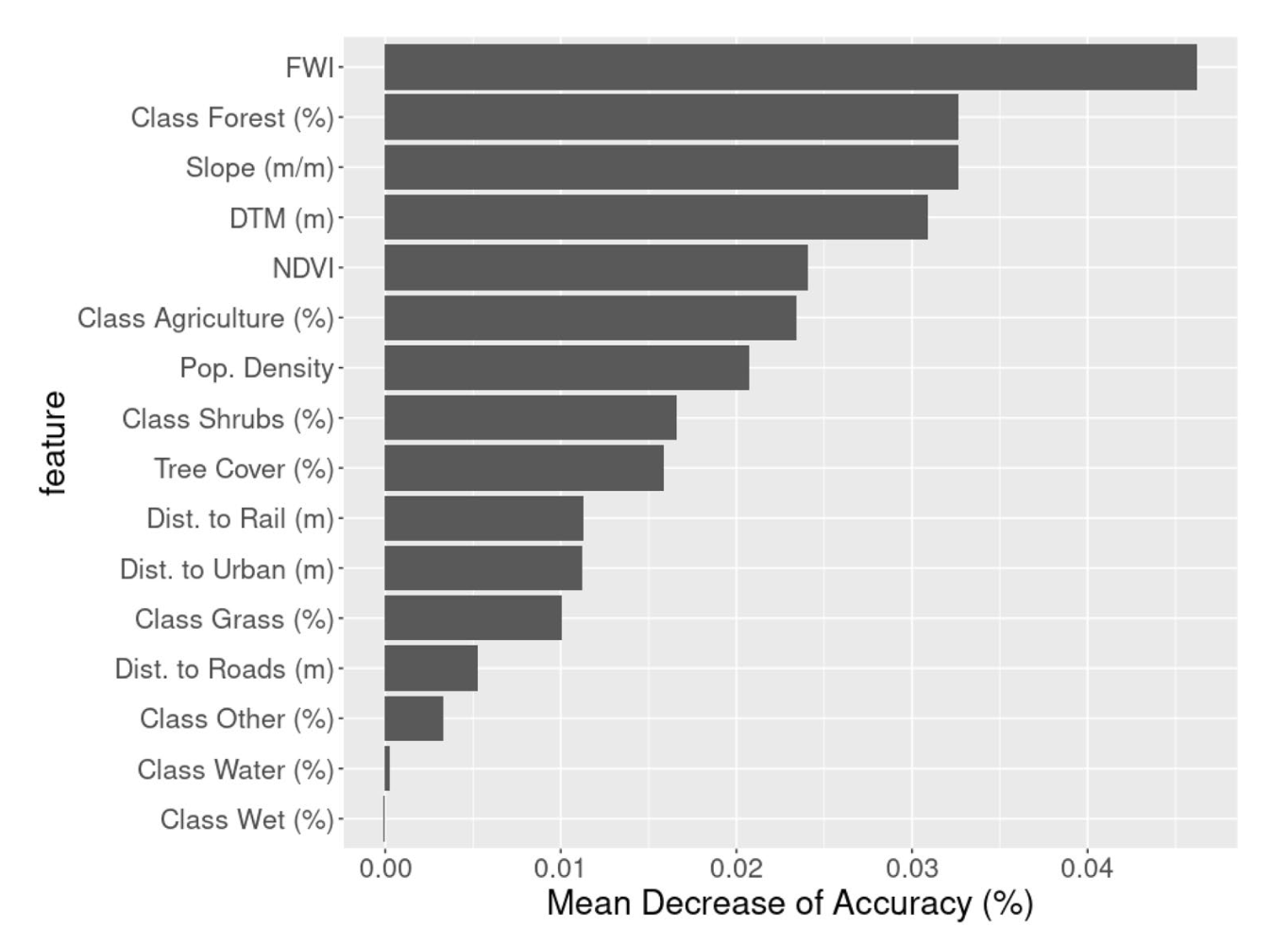
Evaluation of pre‐training large language models on leadership‐class supercomputers
Introduction
The training of large language models (LLMs) is compute intensive and requires large amounts of data. The environmental impact of developing and training LLMs must be kept in mind.
Contributions include:
- Estabilishing performance baselines by benchmarking two LLMs training frameworks
- Developing cost models for runtime and energy projections.
- Drawing insights on future platforms for training LLMs
Two distributed training methods are tested: pytorch's fsdp and Deepspeed
Scaling Laws of Transformers
The accuracy of DL models scales with the amount of data used. The loss of LLMs scales with both the training data and model parameters. Consequently, it scales with the amount of computation.
The total number of floating point operations (FLOPs) is approximately,
\( T_{FLOPS} ∼ 6 \times P \times D\)
where P and D are number of model parameters and tokens, respectively.
Compared to the attention and other blocks, the feed forward block typically requires the most computation. For each element of a feed-forward weight matrix, there are a total of 6 FLOPs per input token. The computation hence scales quadratically with the model size.
For example, training a 175B parameter GPT3 model requires \(3.7×10^{24}\) FLOPs, and it quickly grows to \(1.2×10^{26}\) FLOPs for a 1T parameter GPT-style model.
With fsdp enabled, memory usage per device is:
\( M_A = M_{total} / N_{devices} = 6 * M_p / N_{devices} \)
The per device communication volume per batch step, denoted by C_A, is \(1.5\times \) the one of DDP.
\( C_A ~ 3 \times M_p \)
For DeepSpeed, the memory usage per device is:
\( M_B = \frac{M_p}{PP * TP} + \frac{M_o}{DP} + \frac{M_g}{PP * TP} + M_e \)
So:
\( M_B = \frac{2 * ( DP + PP * TP +1 ) }{N_{devices}} * M_p \)
While the per-device communication volume in each batch step is:
\( C_B ~ (\frac{TP}{N_{devices} + 1}) * 2 M_p \)
Compared to fspd, Deepspeed has better parallelism scalability and can reach better performance when finetuned correctly.
Computational Analysis
The total number of compute operations needed for optimal training of LLMs is quadratically proportional to the number of model parameters.
Runtime and energy projection
the runtime can be straightforwardly predicted via
\( t = T_{FLOPs}∕R_{FLOPs} \) \( ∼ 120 \times P^2∕R_{FLOPs}, \)
where \(T_{FLOPs}\) and \(R_{FLOPs}\) are the compute operations in FLOPs and training performance in FLOPS
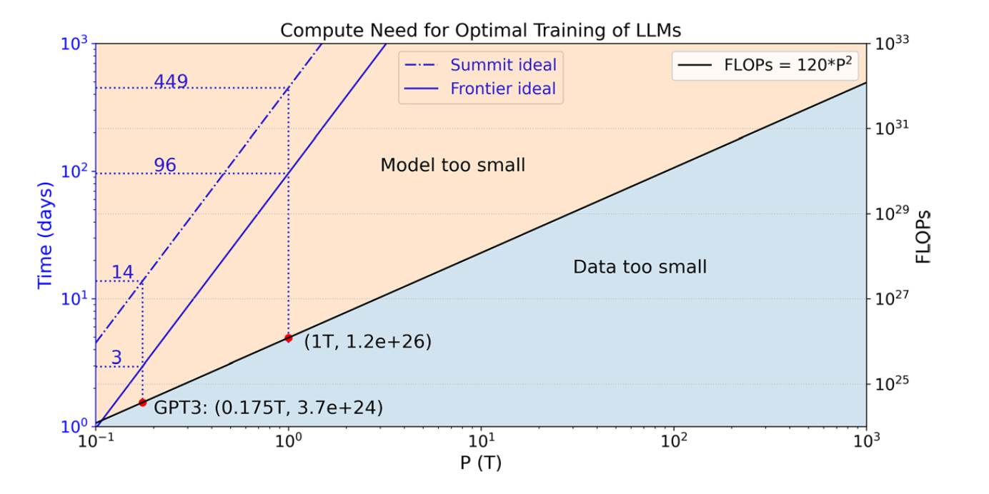
The energy consumption can be evaluated by:
\(E = t \times R_{𝚆𝚊𝚝𝚝}\)
where \(R_{𝚆𝚊𝚝𝚝}\) is the averaged power measured from few iterations.
For Summit and Crusher: the peak performance in half precision for the V100 (112 TFLOPS) and MI250X (384 TFLOPS) GPUs and linear scaling up to full system
Scaling analysis
To evaluate training, both Summit and Crusher (early access testbed for frontier) supercomputers at olcf have been used.
The minimum model-parallel scale required to fit GPT-16B on summit is 2 nodes.
Comparing training of GPT-1.4B and GPT-175B on fsdp and Crusher, the per device performance increases by 17%, indicating there exists a tipping point between the tradeoff of more computation and more communication.
The training performance for FSDP and DeepSpeed-Megatron is 62.1 and 65.1 TFLOPS, respectively. From this baseline, the performance drops 20% and 44% for DeepSpeed-Megatron when using tensor parallelism within a NUMA domain and a node on Summit, respectively. The impact for FSDP is less (30% within a node compared to 44% for DeepSpeed-Megatron) due to less frequent communication and a smaller total message size.
We scale up the LLMs training on both Summit and Crusher:
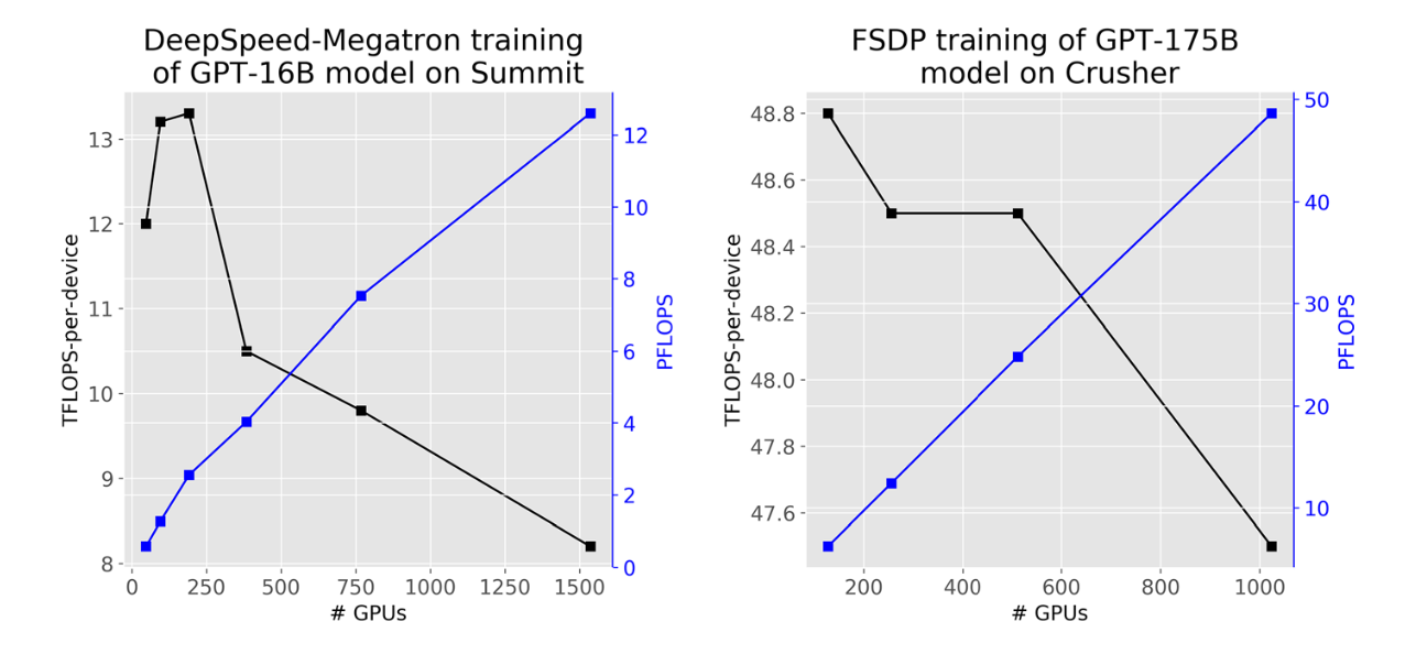
The scaling efficiency is about 97%, signaling Frontier can be a promising platform for training LLMs of these model sizes
Energy consumption
To estimate the energy usage, we trace the GPU power in watts during the training for FSDP training of GPT 175B model on Summit and Crusher. One batch step takes 359 and 301 s, correspondingly.
All processes show periodical behaviour due to the frequent allocation and deallocation of memory to fit large models.
The averaged power usage is about 85 and 408 Watts, for Summit and Crusher, respectively, and the corresponding computational efficiency is 0.165 and 0.235 TFLOPS/Watt.
Similarly, we trained GPT-1T with DeepSpeed on Summit and FSDP on Crusher. One batch takes 341 and 1290 seconds respectively.
Compared to training GPT-175B, the power usage is significantly lower, indicating lower computational loads.
Overall, Crusher is 2 orders of magnitude more efficient than Summit when training GPT-1T model.
As Crusher system bears the same architecture as the first Exascale system Frontier and their unprecedented mix-precision capability, we believe they are well-suited as the platform for training LLMs at extreme scale.
One caveat to consider in our estimation is that the analysis is based on the current implementations of GPT-NeoX (DeepSpeed-Megatron) and PyTorch (FSDP). It’s important to note that the field is rapidly evolving, with ongoing advancements that can further reduce communication costs.
Energy Projections
We projected the trainign time and energy consumption for training GPT-1.4B to GPT-1T on Summit and Frontier.
For larger models, a range is provided with the lower bound being 1x and 20x of the model parameters. Given the per-device computational performance, and the average power, the power efficiency can also be estimated.
It turns out that Crusher is more energy-efficient for training LLMs, and the advatage grows rapidly.
Training LLMs is over 4x more power efficient than executing traditional HPC workloads. (~52 GFLOPS/Watt)
Conclusion
Compared to the theoretical peak performance of a device, there is a gap in how much performance can be achieved in practice when training LLMs, especially at scale. The achievable performance is about 40% of the theoretical peak.
Accomodating a large model comes at the cost of additional communication and the performance at scale has another 3x and 2x orders of magnitude drop for Frontier and Summit respectively. The impact is larger on summit due to the per node memory being 5x smaller and hence more nodes are required to fit the model. Also the node bandwidth is 4x smaller.
For GPT-1T model using a senquence length of 2048 tokens, one GPU can fit 4 samples per batch. The ideal step time for linear scaling is:
\( t^{step} = \frac{T^{step}_{FLOPs}}{R_{FLOPs}} \) \( = 4.9 * 10^4 / R_{FLOPs} \)
The minimum bandwidth required to achieve perfect scaling following communication volume C_A is:
\( b_{ideal}(GB/s) = C_A / t^{step} = 0.24 * R_{FLOPs} \)
For theoretical peak and achievable performance, the minimum per-device communication bandwidth needed is 37 and 94 GB/s, respectively. The current 25 GB/s per-device on Crusher is not sufficient to support linear scaling for training GPT 1T model.
We ignore I/O requirement in our analysis because it can be straightforwardly hidden among computations given the typical global batch size of millions of tokens.
Ideas
-
Graph with Computation need (FLOPs) and ideal training time (days) assuming peak performance and perfect scaling for optimal training of LLMs on Summit and Frontier, respectively. This assumes perfect scaling --> can we do it with estimated scaling from Frontier?
-
Compare real benchmarks with projections from Yin paper
Scaling Laws for Large Language Models
Introduction
Analysis of cross entropy loss for LLMs. It scales as power law with regards to model size N, dataset size D, and amount of computation for training C. Network depth and width have minimal effect on the scaling.
Takeaways
- Performance depends on scale, so number of parameters, amount of data, and amount of computation.
- Performance depends weakly on network depth and width.
- Smooth parameters: performance has a power law dependence with N, D and C.
- Performance is good if \(N \approx D \). Performance penalty depends approximately on the ratio \(N^{0.74}/D\). So by increasing the model size by 8x, we would need 5x the data to maintain performance and avoid penalty.
- These networks are more sample efficient compared to smaller networks.
- Convergence is inefficient, optimal performance is obtained when stopping shortly of convergence.
- Optimal batch size is a power of the loss only. It can be calculated by measuring the gradient noise scale.
Scaling Laws
- \( L(N) = (\frac{N_c}{N})^\alpha_N\) is the loss by keeping the number of parameters fixed. where \(N_c \approx 8.8 \times 10^{13} \) and \(\alpha_N \approx 0.076\). If we increase model size then the dataset size has to be increased linearly, according to \(D \approx N^{0.74}\).
- \( L(D) = (\frac{D_c}{D})^\alpha_D \) is the loss by keeping the dataset size fixed.
- \( L(C_{min}) = (\frac{C^{min}_c}{C^{min}})^{\alpha^{min}_c} \) is the loss by keeping the amount of computation fixed.
Each \( \alpha \) parameter indicates the degree of performance improvement with respect to the parameter.
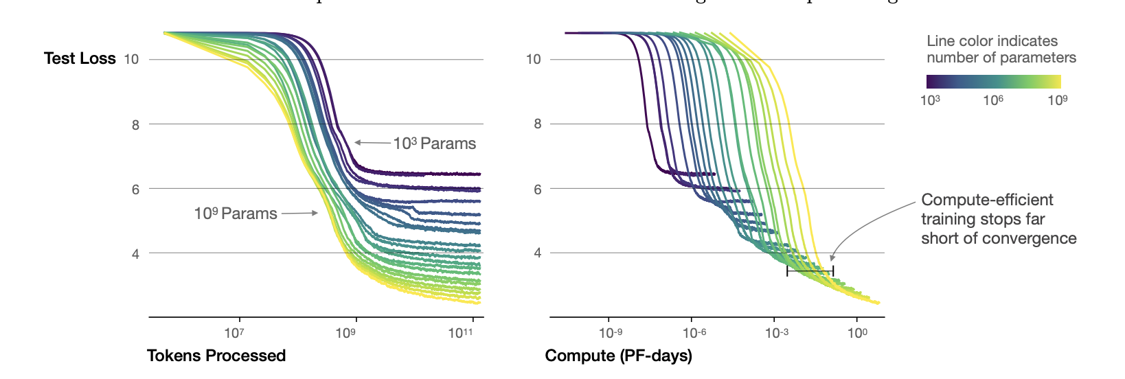
Critical Batch Size
The critical batch size is used for understanding the tradeoff speed-efficiency for data parallel training. It also obeys the power law L.
\( B_{crit}(L) = \frac{B_*}{L^{\frac{1}{\alpha_B}}} \)
where \(B_* \approx 2^{8}\) and \(\alpha_B \approx 0.21 \).
Critical Batch size follows the same scaling laws as performance increases. It needs to be increased by a factor of 2 for every 13% decrease in loss. In the same way, it is indipendent of network depth and width and model size.
\( B_{crit}(L) = E_{min} / S_{min} \)
where \(E_{min}\) is the minimum amount of samples needed to be processed and \(S_{min}\) is the minimum amount of steps needed to reach the L.
Early Stopping
Overfitting is proportional to the correction from ending training at \( S_{stop} \), where \( S_{min} \approx S_{stop} \). Also this needs to be an under-estimation, as test loss decreases slower than training loss.
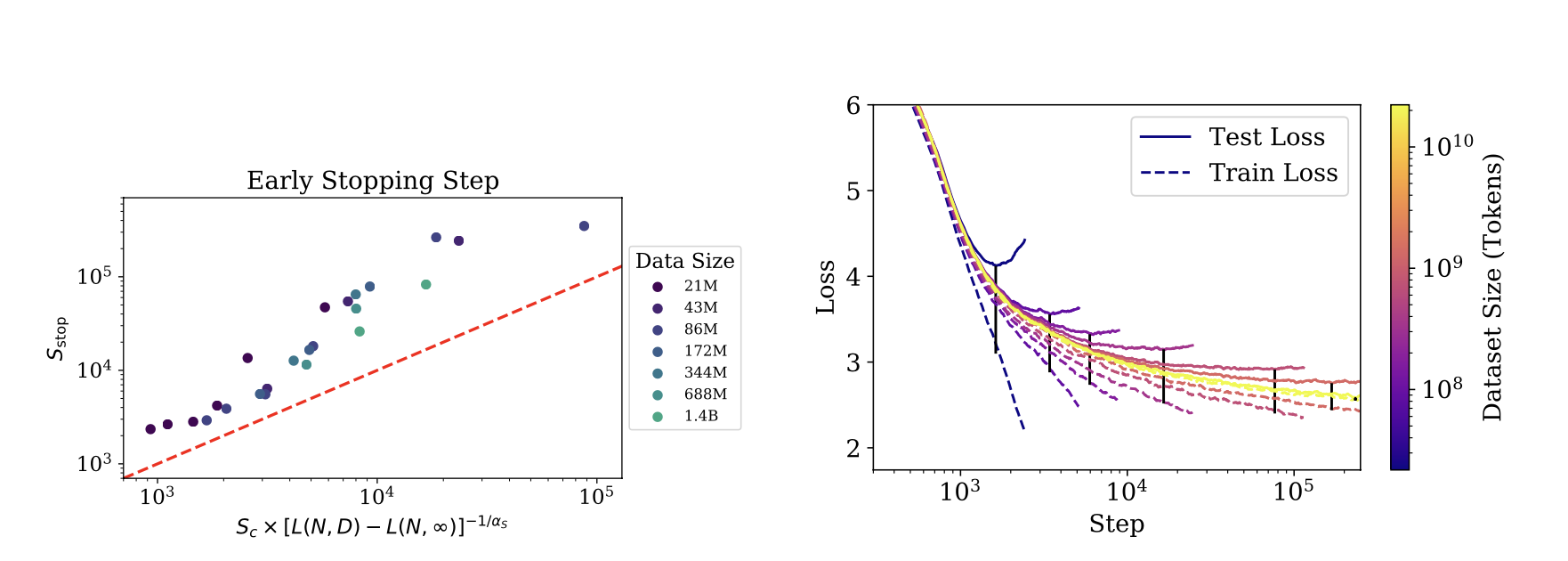
\( S_{stop}(N, D) \geq \frac{S_{min}}{[L(N, D) - L(N, \inf)]^{\frac{1}{\alpha_s}}} \)
where \( L(N, \inf) \) is the converged loss after training on infinite data.
Training Compute-Optimal Large Language Models
Summary
Optimal model size and number of tokens is fixed with the compute budget.
What is found is that model size N and numbe of tokens D should scale equally.
\( 2 \times N \implies 2 \times D \)
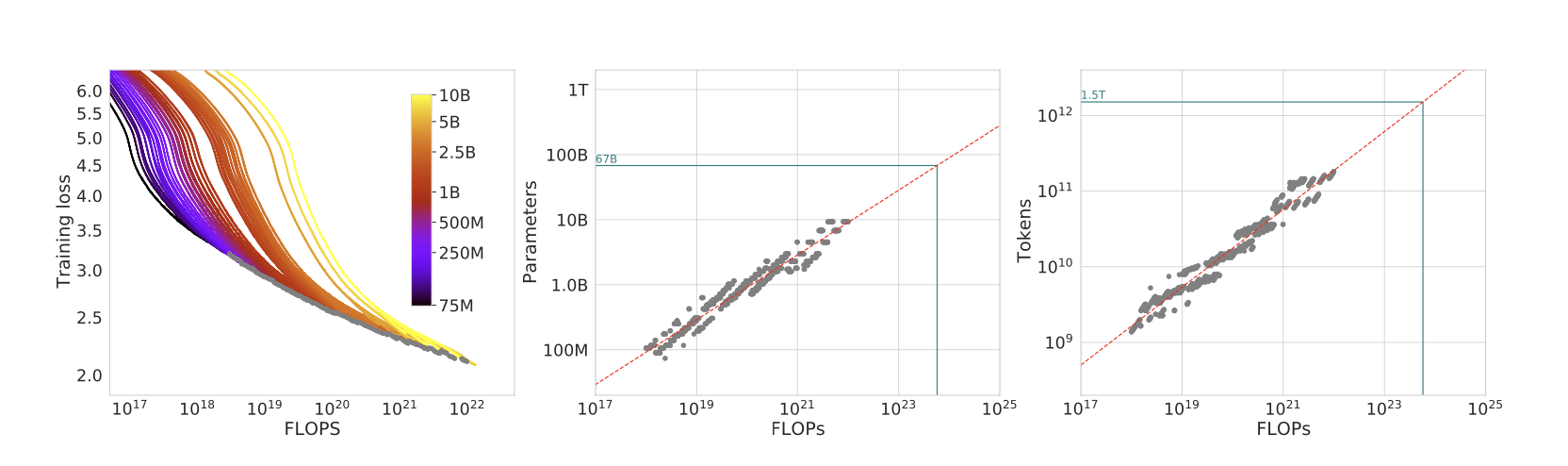
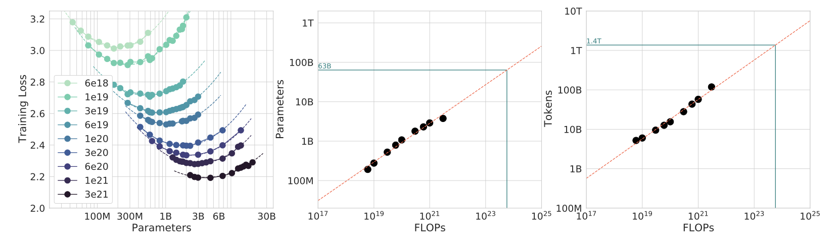
Given a fixed FLOPs budget, how should we tradeoff model size N and training tokens D?
- Fix N and vary D (from 70M to 10B)
- Fix D and vary N (create 16 FLOPs curves (isoFLOPs))
- Fitting a parametric loss function: model all losses as parametric functions of N and D
\( \hat{L}(N, D) = E + \frac{A}{N^{\alpha}} + \frac{B}{N{\beta}}\)
where \(E\) is the entropy of natural text, the second term indicates how a transformer with N parameters still underperforms, and the third term is the finite number of optimization steps.
This function can be optimized with Huber loss, creating M isoFLOPs slices and isoLoss contours.
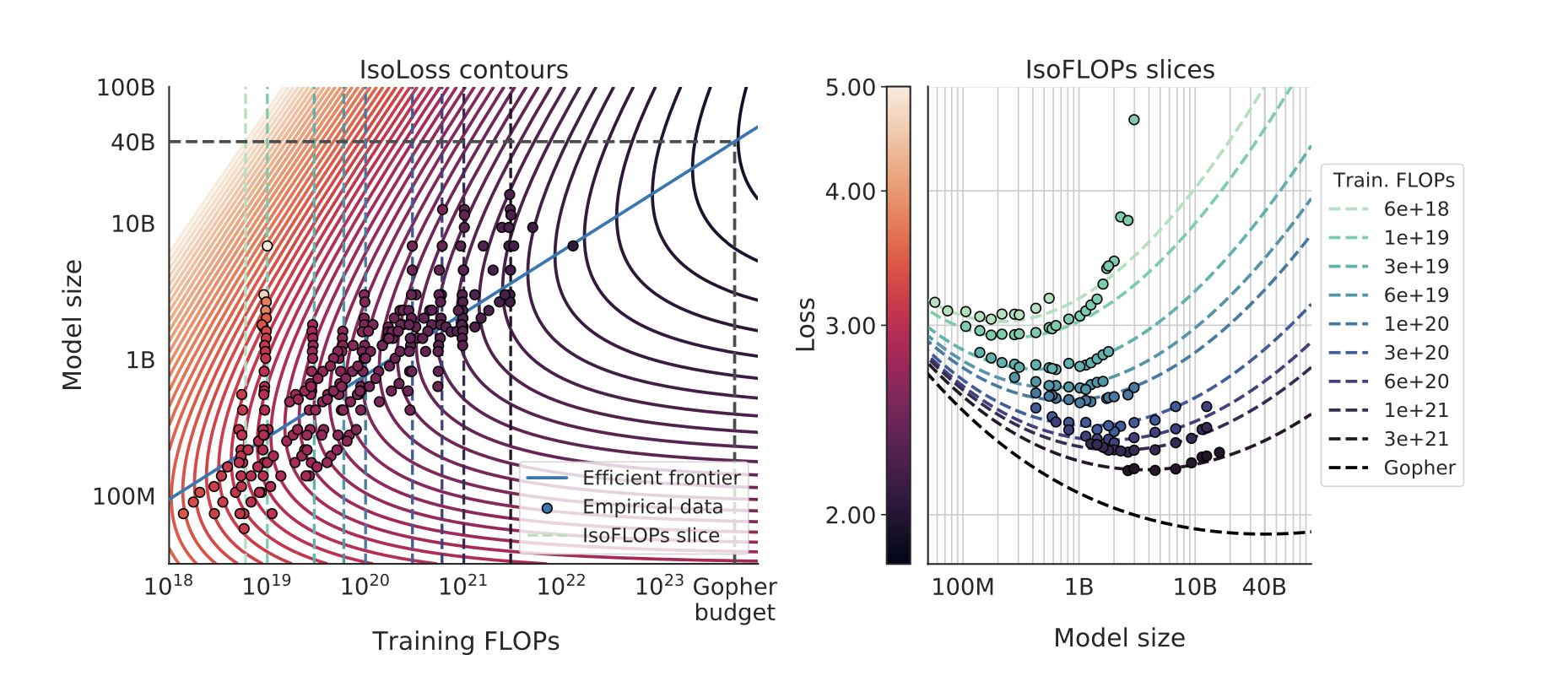
Optimal model scaling?
All three approaches yield the same optimal scaling law: to keep C constant, N and D have to scale in a proportional way.
Scaling Data-Constrained Language Models
Summary
In a data constrained regime [900B, 9B] parameters, with a fixed data and compute budget, after four epochs, the delta in loss is negligible. This implies a decreasing value in repeated tokens.
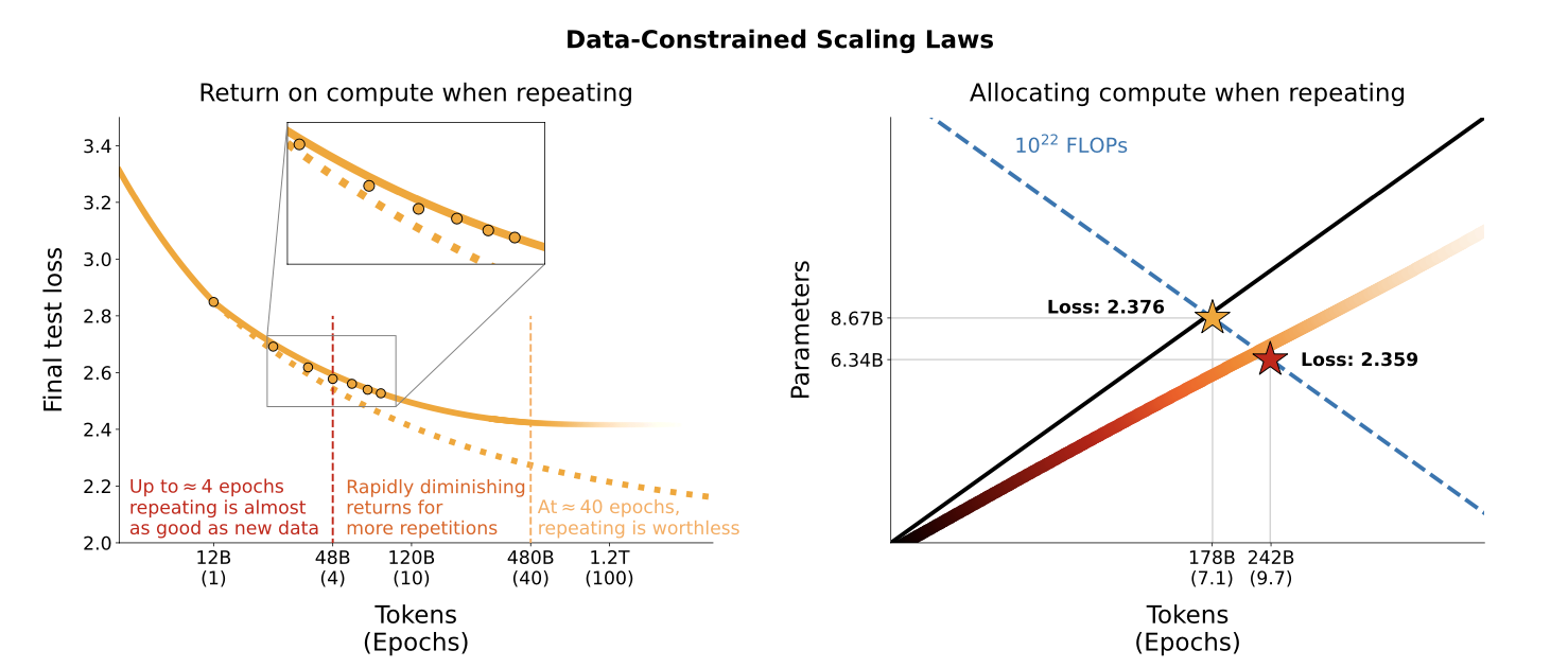
What is the best allocation and return for the given C resources?
- Allocation: how to distribute the compute budget between the model size and the number of training tokens?
- Return: how to measure the gain performance?
Why repeating data? Cause there may not be enough, and it is cheap to generate, but also repetition for the model, that's why we have epochs.
Measure of validation loss for isoFLOPs: too many epochs lead to overfitting. This under any D. For most D sizes, it seems 7 epochs is the best amount.
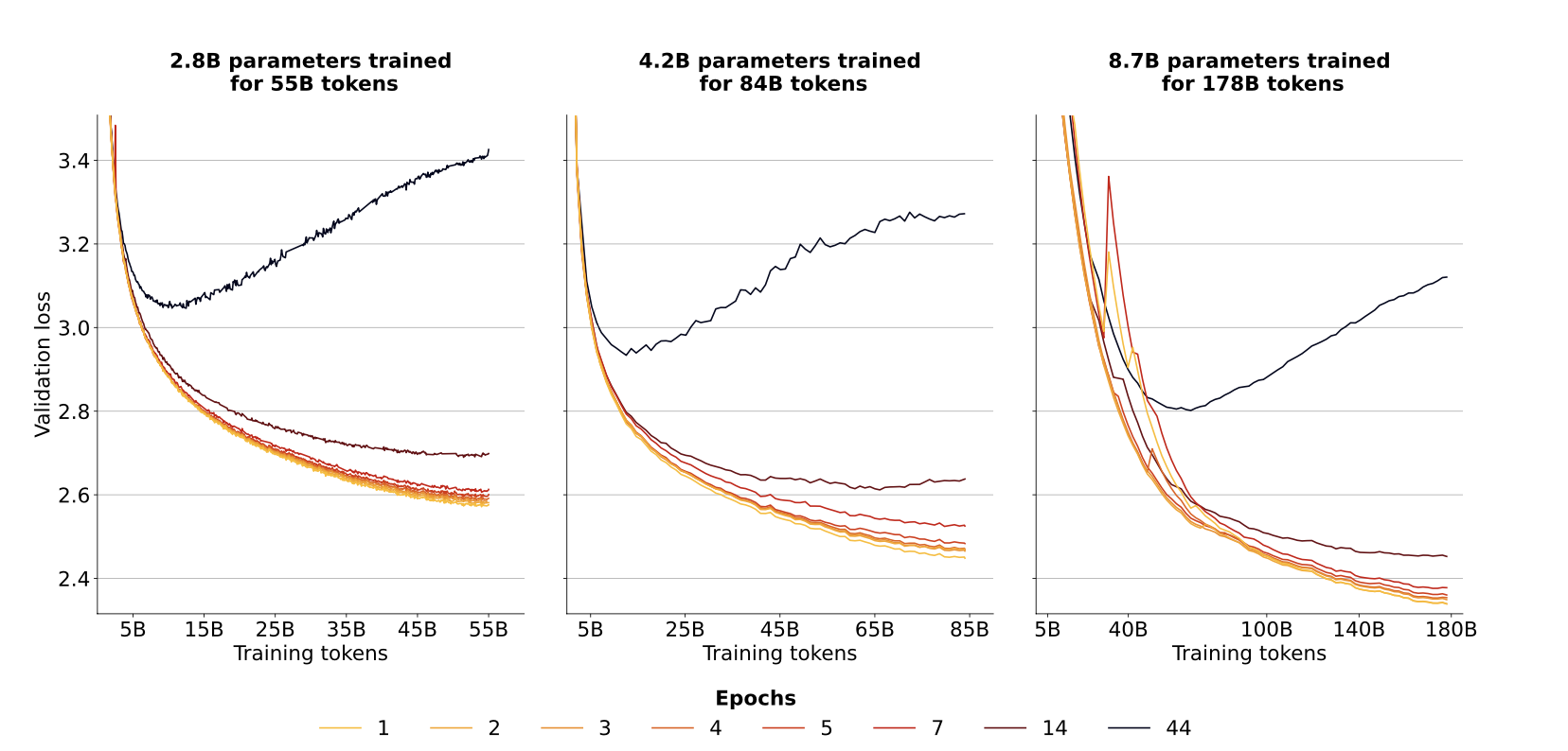
- Allocation: optimized by scaling epochs more than other parameters.
- Return: sizeable when repeating data, after 16 epochs, the gain is negligible.
Scaling laws still hold when repeating several epochs, although with diminishing returns.
Parallelization
Techniques for pytorch
- DDP: the model is copied on all processes, the dataset is split on all the workers and each model is fed a different batch gradient communication is used to keep the models in sync (also overlap of gradient computation)
- RPC: used if training paradigm can’t fit using DDP
- Collective Comms: foundation for RPC and DDP, low level APIs
Paradigms
- Model Parallelism: each worker focuses on a portion of the model, best for large models.
- Data Parallelism: split train set on each worker, shared weights (DDP)
- Parameter server architecture: central node with parameters, workers update the weights by computing the gradient
- All-Reduce Comms: several workers compute private gradient, then combine with all-reduce operation to share global gradient.
- Gradient accumulation: compute gradient on several minibatches, used if comms overhead is high.
Distributed deep learning
Distributed training is the process of subdividing the training workload of, for example, a large neural network across multiple processors. These processors are often referred to as workers, and they are tasked to compute in parallel to speed up the training process. There are two approaches to parallelism: data and model. In data parallelism, the full training set is divided between all the workers, where a copy of the model is also kept. Training is done either synchronously, where all the workers wait for each other, synchronize the gradients, and only then perform the backward step; or asynchronously, where a selected worker is tasked with keeping an updated version of the weights, and all the others can read and write from this worker, often called a ”parameter server”. Using the latter procedure means that all resources are used at the same time, without any delay. However, it also means that only one worker at a time is training with the latest version of the weights. In large clusters the centralized nature of this approach can also create bottlenecks. Model parallelism, on the other hand, divides the model either horizontally, i.e. node-wise, or vertically, i.e. layer-wise, between several workers who are allowed to run at the same time. This approach also reduces the footprint of the model in each worker, making it lighter on the GPU’s memory.
DDP
Distributed Data Parallel is a method of data parallelism that enables a program to operate on numerous machines simultaneously. Applications utilizing DDP generate numerous processes and initialize one DDP instance for each process.
FSDP
In some cases, it may not be possible to create a duplicate of the model for every process. In these instances, Fully Sharded Data Parallel may be utilized, where the optimiser states, gradients, and parameters of the model are subdivided across all DDP ranks. In this case, the neural network is divided into smaller sub-models, each of which represents a portion of the parameters of the overall model. This approach allows different parts of the model to be processed simultaneously by different processing units, and can be used in conjunction with a data-parallel approach that splits the training set to achieve even faster processing times. This results in a program that has less impact on GPU memory, thus reducing execution times.
DeepSpeed
DeepSpeed is a deep learning optimisation suite that enables efficient scalability and faster execution times for both training and inference of large machine learning models. It was developed by Microsoft and claims to offer a 15x speedup over other state-of-the-art parallelization techniques. It provides memory efficient data parallelism and enables training without model parallelism through a novel solution called Zero Redundancy Optimizer. Unlike basic data parallelism, where memory states are replicated across data-parallel processes, ZeRO partitions model states and gradients to save significant memory. Several other memory optimisation techniques are also used, such as Constant Buffer Optimisation, which combines all communication-based operations into a single operand, and Contiguous Memory Optimisation, which reduces fragmentation during training.
Data Quality
The concept of data quality is a complex one. It includes data accuracy, completeness, consistency, timeliness, uniqueness and validity. High quality data depends on the needs of the organization. (highly contextual to the organization).
- Accuracy: it confirms that the data represents the real world.
- Completeness: it ensures that the data is comprehensive of all fields and records.
- Consistency: it ensures that the data is consistent across all systems and databases.
- Timeliness: the delay between data generation and usage doesn't affect accuracy.
- Uniqueness: it ensures that the data is unique and not duplicated.
- Validity: it ensures that the data is in the correct syntax and format.
Fitness for Purpose: find the correct data for your task, otherwise it will be useless for training.
The aim should be to create enterprise wise standards and governance. For example, quality data metric (QDI), which is the percentage of records that are accurate and available across all systems of the enterprise.
Trustworthy AI
Sources:
Introduction
This list provides essential requirements for designing trustworthy AI systems.
- Human agency and oversight: AI systems should complement and empower humans without replacing them
- Technical robustness and safety: AI systems should be technically robust and perform as expected by the users
- Privacy and data governance: AI systems should protect user data and govern its usage at every step of its lifecycle.
- Transparency: The transparency of an AI system refers to the need to explain, interpret, and reproduce its decisions
- Diversity, non-discrimination, and fairness: AI systems should treat all sections of society fairly without discriminating based on factors such as socio-economic determinants
- Societal and environmental well-being: AI systems should not cause any harm to society or the environment during their design, development, and use
- Accountability: AI systems should be able to justify their decisions
TRUSTWORTHY AI REQUIREMENTS
Fairness
Pre-processing models:
- Bias mitigation method for word embedding, which approximates the effect of removing a small sample of training data based on the bias of the resulting system. This system is helpful to trace the origin of the bias in the dataset
- T-closeness technique for discrimination prevention. This technique is helpful to clean data of historical decisions before using it and provides a formal guarantee about the level of discrimination present in the dataset.
In-processing models:
- Fair classifiers using decision boundaries, ensuring fairness concerning one or more sensitive attributes.
- Regression algorithms fair by applying and weighting a regularizer to the standard loss function. This method provides both individual and group fairness and can calculate a numerical value for the effect of fairness on accuracy.
- Bias mitigation method using adversarial learning, which uses the concept of maximizing predictor accuracy while minimizing the ability to predict protected attributes. This method is helpful for both classification and regression tasks
Post-processing models:
- Removes bias by adjusting the learned predictor to balance among supervised learning methods. This method mitigates bias while preserving the privacy of the system.
- Different classifiers for different groups to mitigate bias. This approach is beneficial if all of the groups are not represented equally in the data.
Bias detection methods:
- Test generation mechanism to detect bias in the system. It detects all combinations of protected and non-protected attributes that can lead to discrimination through directed and undirected search.
- Fairness testing approach known as the Flip Test, which tests fairness at the individual level to detect statistical and casual discrimination.
Explainability
Pre-modeling approaches:
- Explaining the datasets on which the system is trained. Researchers proposed visualization techniques to better understand the data before using it.
- Achieve explainable data is through data standardization. Data labeling, in which data is labeled based on its quantitative and qualitative properties
- Creating a data sheet consisting of all information related to the data collection process, dataset features, and recommended use.
In-modeling approaches:
- Utilize the graph structure of trees where internal nodes represent tests on features and leaf nodes represent class labels. Different paths from the root to leaf nodes represent different interpretable classification rules
- Linear models to provide interpretability by visualizing the weight and sign of the features for a given output. This means that if the weight is high and the sign is positive, it will increase the output of the model.
Post-modeling approaches: building proxy models on top of black-box/complex models
-
Feature importance explainability approaches: provide explainability by assigning feature importance values to the input variables. These values reflect which features played more critical role in the decision-making process.
- LIME (Local Interpretable Model-agnostic Explanations), which provides local interpretability to different classifiers and regressors by highlighting essential features that led to the decision.
- LRP (Layerwise Relevance Propagation) for image classification algorithms, which includes interpretability by computing every pixel’s contribution to the prediction made by the classifier. This method utilizes heat maps to visualize the pixel importance.
- SHAP (SHapely Additive exPlanations) method provides interpretability by assigning feature scores to each attribute for different predictions.
-
Example-based explainability approaches: provide explanations and interpretability by creating proxy examples of the model and are based on selecting some instances from the input dataset and monitoring their corresponding outputs to explain the system.
- MMD-critic, which uses both prototype building and criticism selection to provide human-level interpretability. This method claims that prototypes are not enough to give interpretability to complex black boxes.
- Providing counterfactual explanations that describe only the most essential variable that led to a decision and how a slight change in that variable can lead to a completely different outcome.
-
Rule-based explainability approaches: rule-extraction techniques to give comprehensibility to artificial neural networks. These techniques provide a comprehensive description of the knowledge learned in the training phase using the system’s input and output
- TCAV (Testing with Concept Activation Vectors), which uses the internal state of neural networks to provide interpretability
-
Visualization-based explainability approaches: offer explainability by visualizing the internal working of opaque AI systems
- Visualizing how the change in the feature importance affects the model performance.
- Visualizing the contribution of the evidence for the final decision to provide explainability to classifiers
Accountability
Algorithmic accountability includes assessing the algorithms based on various parameters and assigning responsibilities of harm to different stakeholders involved in developing the algorithms.
Ex-Ante methods: before the actual development of the algorithms and mainly deal with the algorithms’ planning and design phase, which helps assign responsibilities for the decisions made by the algorithm even before its actual development.
- Assign different priorities to different algorithm values through discussion between various stakeholders and the public council. This method will help algorithms resolve conflicting issues through prioritization, which prevents harm and will lead to better governance and accountability. The one drawback of this type of method is that it is difficult for people with different interests to agree on a single design.
- Laying out all the design specifications and clearly describing what the system is intended to do in different circumstances enforces better governance and accountability.
- Time frame mechanism in the design process that prevents harm by timely reevaluating the system to ensure it is working as per the prior specifications and guidelines. This timely checking of the system will help governance and increase the user’s trust in the system.
In-Ante methods: implementing accountability measures in the development lifecycle of the AI system itself and ensure that AI systems are developed as specified in the planning and design phase
- Ensure that the data used for training is diverse and does not have any bias
- Guarantees that an appropriate model has been chosen based on the problem requirements
- Ensure that proper testing is done before deploying the system
Total transparency could lead to many adverse effects like loss of privacy, loss of trade secrets, and more attacks. There can be cases where total transparency can lead to less answerability. Because of these side effects, they proposed that total transparency for accountability should not be provided to the general public but only to the oversight agencies the public should trust
Post-Ante methods: providing accountability measures after the model is deployed.
- legal framework to ensure that the deployed model works within the specified boundaries
- ethical algorithm audit that can be used for external validation of the system, helping the deployed system to be free from biases and errors and safe to use
- algorithmic auditing technique to detect algorithmic bias in the system. They discussed how auditing techniques would help operationalized bias mitigation methods and lead to the development of fair algorithms
Privacy
Some researchers have proposed federated learning to provide privacy to the user data using the concept of collaborative learning where the raw data is not shared among the devices; instead, the model is shared after being trained on local devices.
- Distributed learning method that uses data stored on mobile devices to compute a shared learning model, which prevents the need to centralize data storage providing data privacy as data is distributed over users’ mobile devices.
- PEFL (Privacy Enhanced Federated Learning) approach, a non-interactive approach that can prevent data leaks when different entities interact.
Provenance Documentation for Trustworthy AI
Summary
AI models should be transparent, explainable and trustworthy (TAI), using provenance to explain complex models. Provenance answers questions who-what-where to obtain reproducibility, trustworthiness and explainability. The idea is to be able to understand the metadata and the provenance of ML artifacts. (FATE in AI --> there is no roadmap yet)
Trustwothy AI: AI-based system that are lawful, ethical and robust in the face of adversarial attacks. This is to estabilsh XAI (Explainability). Some examples are DARPA XAI program, HLEG EU program (guidelines on AI).
Post-Hoc Explainable techniques:
- Model specific: TSHAP, DeepLIFT, Grad-CAM
- Model agnostic: LIME and SHAP
Provenance documentation is still necessary to complement XAI, increasing transparency with:
- How data is collected
- Data ownership and rights
- Trace steps in data analysis
Tools for provenance documentation:
- W3C PROV anthology
- W3C PROV Data model (PROV-DM): web anthology language (PROVN) OWL2
Tools for validation and browsing of provenance documents:
- PROV validator, Prov Viewer
- Common workflow language (CWL) also for ML
- PROV-JSON, OpenML, Model-DB
- prov-py allows to export provenance information from Python scripts
- Jupyter to automatically generate provenance information with packages and reproducibility
Information Required for XAI
Summary
Introduction of a 6-w framework to create a graph based system to provide user with information about training and data used by the ML model.
Open Issues:
- Requirements for XAI decision support systems --> What info does the user need to make a decision?
- Can the user check all steps for an answer from the model?
- Security evidence of an AI system? Are there biases (even deliberate)? Safety Mismatches, Misrepresentations?
Informtion required for XAI:
- Human point of view --> ML systems are not transparent even for experts or designers
- Security point of view --> generated explanations can be misleading (deliberate manipulation of the results)
Provenance information: PROV-DM model, keeps history of data records, provenance linking of Input and Output of an AI system.
6W framework for provenance graph XAI design:
- Who: user, developer, data generation, modification and explanation
- Where / When: process, system and design
- Why: Governance, policies and laws
- What: Data, documents, decision, system information
- Which: security, safety information and protocol
TODO: WRAPPER AROUND AI MODEL CONTAINING INFO ABOUT TRAINING PROCESS, DATASET USED (STD, MEAN, VARIABLES --> IF INFO ABOUT DS ARE NOT MATCHING THEN PROBLEM?). HASH FUNCTION TO DETERMINE IF THE PROCESS OR RESULTS HAVE BEEN MANIPULATED. TODO: PROVIDE PREVIOUS RECORDS OF SIMIL. INPUT AND GT (THIS REQUIRES THE FULL DATASET), OTHERWISE JUST VARY THE INPUT SLIGHTLY TO SEE CERTAINTY AND POSSIBLE PIVOTAL FEATURES
Explainable AI Techniques
Introduction
EXplainable Artificial Intelligence (XAI) techniques can serve to verify and certify model outputs and enhance them with desirable notions such as trustworthiness, accountability, transparency and fairness.
Explainable AI Techniques
Explanations
SHAP
SHAP (SHapley Additive exPlanations) is a model agnostic approach which decomposes the output of a model among all its input features. It is based on Shapley values from game theory. It performs an additive feature attribution analysis:
\( g(x) = \omega_0 + \sum_i^M{\omega_i x_i} \)
where \( \omega_0 \) is the expected value of the model output as baseline, \( \omega_i \) is the contribution of feature \( i \) and \( x_i \) is the value of feature \( i \).
SHAP has two inner models for each feature i, then computes the difference between both models' outputs. The difference is the contribution of feature i. The model yields the estimated feature importance by perturbing the input features and observing the change in the output.
This method can visualize how much each feature changes the output of the model.
This method only focuses on a model's inner functioning, no alignment with human expert explanation and reasoning is made.
DiCE
DiCE (Diverse Counterfactual Explanations) is a model agnostic approach which generates counterfactual explanations from a set of events, given a model and a query.
This becomes an optimization problem, where the objective function is the distance between the counterfactual and the original instance.
The final distance is calculated as a function of:
- Diversity: encoded as the determinant of the covariance matrix of the counterfactual explanations
\( dpp_diversity(K) = det(K) \)
where: \( k = \frac{1}{1+dist(C_i, C_j)} \) and \( C_i \text{and} C_j \) are counterfactual explanations.
- Proximity: encoded as negative distance betweeen CFs features and the original input.
\( P = - \frac{1}{k} \sum_i dist(C_i, x) \)
The final set of k CFs for the sample x is obtained by solving the following optimization problem:
\( C(x) = argmin { \sum_k yloss(f(C_i, x)) + \sum dist(C_i, x) - \sum_k dpp_diversity(C_1, ..., C_k) } \)
This method works well even for non-tech audiences. But only works for differentiable models, as it uses gradient descent.
GradCAM
GradCAM (Gradient-weighted Class Activation Mapping) is a model agnostic approach which generates a heatmap of the input image, highlighting the regions that are important for the model's prediction. Gradients from any target create a localized map, which highlights the important regions for the target. This translates to which part of the image contributes more to the model's prediction.
Class Discriminative Localized map:
\( \alpha_k^c = \frac{1}{Z} \sum_i \sum_j \frac{\Delta y^c}{\Delta A_{i, j}^k} \)
where \( \alpha_k^c \) is the importance of feature map (neuron importance) \( k \) for class \( c \), \( \Delta y^c \) is the change in class score (gradient for class c) and \( \Delta A_{i, j}^k \) is the change in activation map \( k \) at location \( (i, j) \).
This method offers a visual explanation. Lacks high resolution heatmap.
Transformer Interpret
Transformer Interpret is a model agnostic approach which is created ad-hoc for transformers. It is based on the attention mechanism of transformers, using the integrated gradents to map the importance of each token to the model's output.
- Sensitivity: if a modification of a feature leads to a change in the classification output, then attribution is different from 0. The feature played a role in the classification.
- Implementation invariance: attribution method should not depend on model parameters.
Integrated gradients adds sensitivity to the gradient based method by having a baseline. This way the model knows how the change in input influences the classification.
This method can be used to interpret positive and negative attributions in output.
LRP
LRP (Layer-wise Relevance Propagation) produces a heatmap for every input data sample, highlighting the regions that are important for the model's prediction.
This method is good for any type of data.
LTN
LTN (Logic Tensor Networks) is a model agnostic approach which is based on first order logic. It is a neural-symbolic approach, which combines neural networks and symbolic reasoning. It involves costraint-based learning with FOL.
It guaranties eterative exploration by saving each model parametrization, just by querying the model for an output.
It tries to synthetize the model's reasoning with FOL. For each step of the network, it approximates the output of the network with a FOL formula.
TS4NLE
TS4NLE (Template System for Natural Language Explanations) is a model agnostic approach which generates natural language explanations for a given model and input.
It is a technique to convert the explanation of an XAI to a natural language explanation. Can also be tailored to a specific domain or audience type.
Provenance
Provenance is information about entities, activities, and people involved in producing a piece of data or thing, which can be used to form assessments about the data or thing's quality, reliability or trustworthiness.
The goal of PROV is to enable the wide publication and interchange of provenance on the Web and other information systems. PROV enables one to represent and interchange provenance information using widely available formats such as RDF and XML.
At its core is a conceptual data model (PROV-DM), which defines a common vocabulary used to describe provenance.
To help developers and users express valid provenance, a set of constraints (PROV-Constraints) are defined, which can be used to implement provenance validators. This is complimented by a formal semantics (PROV-SEM). Finally, to further support the interchange of provenance, additional specifications are provided for protocols to locate and access provenance (PROV-AQ), connect bundles of provenance descriptions (PROV-Links), represent dictionary style collections (PROV-Dictionary) and define how to interoperate with the widely used Dublin Core vocabulary (PROV-DC).
JSON-LD allows a semantic structure to be overlaid over a JSON structure, thereby enabling the conversion of JSON serializations into linked data.
PROV-JSONLD, a serialization of PROV that is compatible with PROV-DM and that addresses all of our 4 key requirements:
- Lightweight: A serialization MUST support lightweight Web applications.
- Natural: A serialization MUST look natural to its targeted community of users.
- Semantic: A serialization MUST allow for semantic markup and integration with linked data applications.
- Efficient: A serialization MUST be efficiently processable.
PROV Data Model
The PROV data model (PROV-DM) is a generic data model for provenance that allows domain and application specific representations of provenance to be translated into such a data model and interchanged between systems.
It distinguishes core structures from extended structures: core structures form the essence of provenance information, and are commonly found in various domain-specific vocabularies that deal with provenance or similar kinds of information. Extended structures enhance and refine core structures with more expressive capabilities to cater for more advanced uses of provenance.
Provenance describes the use and production of entities by activities, which may be influenced in various ways by agents.
An entity is a physical, digital, conceptual, or other kind of thing with some fixed aspects; entities may be real or imaginary. An activity is something that occurs over a period of time and acts upon or with entities; it may include consuming, processing, transforming, modifying, relocating, using, or generating entities.
Communication is the exchange of some unspecified entity by two activities, one activity using some entity generated by the other.
A derivation is a transformation of an entity into another, an update of an entity resulting in a new one, or the construction of a new entity based on a pre-existing entity.
An agent is something that bears some form of responsibility for an activity taking place, for the existence of an entity, or for another agent's activity. Attribution is the ascribing of an entity to an agent. An activity association is an assignment of responsibility to an agent for an activity, indicating that the agent had a role in the activity. Delegation is the assignment of authority and responsibility to an agent (by itself or by another agent) to carry out a specific activity.
The Open Provenance Model
Introduction
Interest for provenance in the “e-science community” is also growing, since provenance is perceived as a crucial component of workflow systems.
Open Provenance Model, a model for provenance which meets the following requirements:
- To allow provenance information to be exchanged between systems, by means of a compatibility layer based on a shared provenance model.
- To allow developers to build and share tools that operate on such provenance model.
- To define the model in a precise, technology-agnostic manner.
- To support a digital representation of provenance for any “thing”, whether pro- duced by computer systems or not.
- To define a core set of rules that identify the valid inferences that can be made on provenance graphs.
Entities
Our primary is concern is to be able to represent how “things”, whether digital data such as simulation results, physical objects such as cars, or immaterial entities such as decisions.
Hence, from the perspective of provenance, we introduce the concept of an artifact as an immutable piece of state; likewise, we introduce the concept of a process as actions resulting in new artifacts. A process usually takes place in some context, which enables or facilitates its execution.
Definition 1 (Artifact) Immutable piece of state, which may have a physical embodiment in an physical object, or a digital representation in a computer system.
Definition 2 (Process) Action or series of actions performed on or caused by artifacts, and resulting in new artifacts.
Definition 3 (Agent) Contextual entity acting as a catalyst of a process, enabling, facilitating, controlling, affecting its execution.
Dependencies
A provenance graph aims to capture the causal dependencies between the abovementioned entities. Therefore, a provenance graph is defined as a directed graph, whose nodes are artifacts, processes and agents, and whose edges belong to one of following categories.
Definition 4 (Causal Relationship) A causal relationship is represented by an arc and denotes the presence of a causal dependency between the source of the arc (the effect) and the destination of the arc (the cause). Five causal relationships are recognized: a process used an artifact, an artifact was generated by a process, a process was triggered by a process, an artifact was derived from an artifact, and a process was controlled by an agent.
Definition 5 (Artifact Used by a Process) In a graph, connecting a process to an artifact by a used edge is intended to indicate that the process required the availability of the artifact to complete its execution.
Definition 6 (Artifacts Generated by Processes) In a graph, connecting an artifact to a process by an edge wasGeneratedBy is intended to mean that the process was required to initiate its execution for the artifact to be generated.
Definition 7 (Process Triggered by Process) A connection of a process P2 to a pro- cess P1 by a “was triggered by” edge indicates that the start of process P1 was required for P2 to be able to complete.
Definition 8 (Artifact Derived from Artifact) An edge “was derived from” between two artifacts A1 and A2 indicates that artifact A1 may have been used by a process that derived A2.
Definition 9 (Process Controlled by Agent) The assertion of an edge “was controlled by” between a process P and an agent Ag indicates that a start and end of process P was controlled by agent.
Roles
A role is an annotation on used, wasGeneratedBy and wasControlledBy.
Definition 10 (Role) A role designates an artifact’s or agent’s function in a process.
Provenance Notation
PROV-N adopts a functional-style syntax consisting of a predicate name and an ordered list of terms. All PROV data model types have an identifier. All PROV data model relations involve two primary elements, the subject and the object, in this order.
The grammar is specified using a subset of the Extended Backus-Naur Form (EBNF) notation, as defined in Extensible Markup Language (XML).
EBNF specifies a series of production rules (production). A production rule in the grammar defines a symbol expr (nonterminal symbol) using the following form:
expr ::= term
Symbols are written with an initial capital letter if they are the start symbol of a regular language, otherwise with an initial lowercase letter. A production rule in the grammar defines a symbol
::= term
Almost all expressions defined in the grammar include an identifier. Most expressions can also include a set of attribute-value pairs, delimited by square brackets. Identifiers are optional except for Entities, Activities, and Agents. Identifiers are always the first term in any expression.
-
Communication
-
Invalidation
-
Derivation / Revision / Quotation
Provenance Constraints
PROV statements involve identifiers, literals, placeholders, and attribute lists. Identifiers are, according to PROV-N, expressed as qualified names which can be mapped to URIs. However, in order to specify constraints over PROV instances, we also need variables that represent unknown identifiers, literals, or placeholders. These variables are similar to those in first-order logic. A variable is a symbol that can be replaced by other symbols, including either other variables or constant identifiers, literals, or placeholders.
Several definitions and inferences conclude by saying that some objects exist such that some other formulas hold. Such an inference introduces fresh existential variables into the instance. An existential variable denotes a fixed object that exists, but its exact identity is unknown. Existential variables can stand for unknown identifiers or literal values only; we do not allow existential variables that stand for unknown attribute lists.
Some placeholders indicate the absence of an object, rather than an unknown object. In other words, the placeholder is overloaded, with different meanings in different places.
An expression is called a term if it is either a constant identifier, literal, placeholder, or variable.
Substitution
A substitution is a function that maps variables to terms. Concretely, since we only need to consider substitutions of finite sets of variables, we can write substitutions as:
\([x_1 = t_1,...,x_n = t_n] \)
can be applied to a term by replacing occurrences of \(x_i \text{with} t_i\).
Formulas
For the purpose of constraint checking, we view PROV statements as formulas.
An instance is analogous to a "theory" in logic, that is, a set of formulas all thought to describe the same situation. The set can also be thought of a single, large formula: the conjunction of all of the atomic formulas.
The definitions, inferences, and constraint rules in this specification can also be viewed as logical formulas, built up out of atomic formulas, logical connectives and quantifiers.
In logic, a formula's meaning is defined by saying when it is satisfied. We can view definitions, inferences, and constraints as being satisfied or not satisfied in a PROV instance, augmented with information about the constraints.
Unification is an operation that takes two terms and compares them to determine whether they can be made equal by substituting an existential variable with another term.
Interoperability with PROV-JSON for Provenance aware databases
Introduction
The PROV standard has been widely adopted as a standardized exchange format for provenance information. However, adaptation for provenance aware databases is still lacking. Here operations of import, export, query and visualization of provenance information are discussed for graph databases (GProM).
With PROV it is possible to track the provenance of an entity during its entire lifecycle.
A Graph Model of Data Provenance
Introduction
Provenance in databases has been defined for relational or complex object data, by propagating fine-grained annotations from the input to the output. Workflow in provenance aims to capture the complete description of evaluation of a process, which is crucial in verification of a scientific computation. Workflows and their provenance are often represented as directed acyclic graphs, but complicating the semantic that relates to the workflow of provenance and their runtime behaviour. This part is often achieved with extended data-flow languages.
The open provenance model has been developed as an exchange format for representing provenance graphs.
A common language to express both databases queries and workflows is necessary. In this case Dataflows (DFL) was used.
In this work, a semantic that evaluates dataflow calculation expressions to provenance graphs containing values, evaluation nodes and links showing how the expression is evaluated is presented; as well as a precise implementation of this model.
Dataflow Language
DFL is a language for expressing dataflow computations, and it is a generalization of the relational algebra. It is an extension of the NRC dataflow language, that only includes atomic values and functions.
Both DFL and NRC are statically typed languages.
Value, Evaluation and provenance graphs
DFL expressions are normally evaluated over complex values, which are nested as a combination of atomic data values d, tuples of complex values \( < A_1 : v_1, \dots , A_n : v_n > \), and sets of complex values \( { v_1, \dots , v_n } \). Complex values can be easily represented as trees or DAGs.
Using value graphs we represent the evaluation of a DFL expression, and using provenance graphs, which are two-sorted graphs consisting of a value graph and an evaluation graph, we represent the evaluation of a program.
Value Graphs
A value graph is a DAG, with labels on the nodes and edges. The nodes are labeled with alphabet \( {{}, <>, \text{copy}}\), while the edges are labeled with the names of the attributes of the complex value. The formula \( lab_l(n) \) is used to indicate that the label of node \( n \) is \( l \) in the graph \( G \).
A tree shaped value graph is called a value tree, and one can always represent any complex values by the root node of a value tree.
Evaluation Graphs
An evaluation graph \( G = (V, E) \) is a labelled directed acyclic graph, with nodes and labeles drawn from the set
\( {x, c, f, <>, \pi_A, let_x, if, for_x, \dots} \)
and optional edge labels drawn from the set:
\( {A, head, body, test, then, else, 1, 2, \dots} \)
A valid evaluation graph is a graph constructed using specific rules (see paper), and can be extended by attaching new nodes and edges or by linking existing nodes.
Provenance Graphs
A provenance graph \( G = (V, E) \) is a DAG containing nodes and edges, with either a value or an evaluation label. It indicates the evaluation of a DFL expression, and is a two-sorted graph consisting of a value graph and an evaluation graph.
Given a provenance graph G and an evaluation node e, there is a notion \((G, e) \) of the node being locally consistant, with the intuition that the computation depicted in the part of the evaluation graph reachable from e matches the assignemnt of value nodes to evaluation nodes by the val-edges.
It is possible to enforce local consistency by using first order constraint on a provenance graph. Global consistency can also be defined by induction on the structure of an expression.
Provenance Graph Semantics
To construct a consistent provenance graph we need to evaluate DFL expressions to construct both value and evaluation graphs.
(See rules in paper)
The rules can be applied to build a provenance graph bottom-up.
Given an ordinary assigment, we can always construct a graph G that defines value nodes for the values the variable and whose evaluation nodes correspond exactly to the values in X.
Querying Provenance Graphs
The provenance graph is a relational structure and as such it can be queried from simple paths to complex queries.
It still seems to be a challenge to define known forms of provenance in databases in terms of provenance graphs. In this work, Datalog is used to define the semantics of provenance graphs.
When and Why Provenance
In order to define forms of where and why provenance, we need to define a partial order on evaluation nodes. Where and Why provenance will be defined on tuples \( (e, v) \) such that v is reachable from e by a directed path. These pairs will be called instances.
The where-provenance can be defined as follows:
\( Where((e_1, v_1), (e_2, v_2)) \leftarrow Before(e_1, e_2), Copy(v_2, v_1) \)
meaning that the provenance of v_2 returned by the evaluation ending at e_2 is the same as that of value v_1 returned by the evaluation ending at e_1. There should be a unique (e_1, v_1) with respect to Before, so we can define the where-provenance as the instance (e_1, v_1).
The why-provenance on the other hand is defined using witnesses. The witness to the existence of a part p of the output of a query on input data d is a subtree of the input d such that re-running Q on the subtree still produces a as output the part p. Let G be the provenance graph with a distinguished evaluation node r and a value node v, let U be a connected subset of the result value node that contains v. Then a witness to U in G is a consistent subgraph of G that contains U and r.
The Why-provenance of V is then the set of all minimal witnesses to U in G.
Provenance Supporting Hyperparameter Analysis in DNNs
Introduction
Deep Neural Networks (DNNs) are widely used in various applications, including image recognition, natural language processing, and climate modeling. The performance of DNNs is highly dependent on the choice of hyperparameters, such as the learning rate, batch size, and the number of layers. The choice of hyperparameters can significantly affect the performance of DNNs, and it is often challenging to determine the best hyperparameters for a given task. In this document, we discuss the importance of provenance in supporting hyperparameter analysis in DNNs.
Techniques
Automatic approaches
- ModelDB: focuses on SparkML and Scikit-learn models, automatically tracks models in their native environments, storing results t oallow for visualization and exploration. Allows only for post-mortem analysis of the pipeline (no runtime provenance analysis).
- Runaway: manages ML and DL artifacts, experiments and provenance. Tracks model and data for reproducibility and provenance. Is restricted to only python3.
- ModelKB (knowledge base): automatically extracts metadata artifacts from ML models. Automatically manages experiments, viewing and consulting. The issue is that there is no runtime provenance analysis.
- Shelter: Automated tool to extract metadata from ML models. Features an interactive view, querying of data and comparison of experiments. It does not follow W3C PROV standards.
Domain agnostic approaches
- NoWorkflow: captures and stores provenance data from python scripts. Doesn't support distributed or parallel execution.
- SPADE: same to NoWorkflow, but also includes support for parallel and distributed execution. It needs to be compiled with LLVM. The process consists in first automatically collecting data, then the used decides how to process. (no control over the type of data collected)
- DFAnalyzer: also allows the user to decide what to collect, but it is not automatic.
- Sumatra: captures data based on annotations in the script (only post mortem analysis).
- YesWorkflow: also annotations in the script, but no runtime provenance.
- UML2PROV: uml based provenance collection, automatically allows for provenance aware apps. Has limited use in many ML environments.
Also tensorflow and keras have their own provenance tracking tools, but only post mortem.
DNN specific approaches
- KerasProv: extends DfAnalyzer to support Keras models. It is also in-situ. Represents data in a way which follows W3C PROV standards. Can also create diagrams with pygraphviz.
FAIR Guiding Principles
Introduction
The FAIR guiding principles are data principles for guidelines to enhance the reusability of code and data.
How to obtain good data management?
Guide the data producers as they navigate the flow of data from the point of creation to the point of publication. To maximize added valueì, all components must be available, and gurantee reproducibility and transparency.
Principles
-
Findability: to be foundable, data must have a global unique identifier, have rich metadata, and be registered or indexed in a searchable resource.
-
Accessibility: data must be retrievable by their identifier using a standard protocol, and the metadata must be accessible even when the data is no longer available. The protocol must be open, free, and universally implementable, and allow for authentication if the process needs it to.
-
Interoperability: data must be able to be integrated with other data, and be able to be used by a variety of applications. Data must include qualified access to other metadata, as well as to follow FAIR principles.
-
Reusability: data must be well-described, and have a rich metadata. It must be described with a plurality of different relevant attributes, have clear and accessible licence, detailed provenance, and meet domain-relevant community standards.
All principles are implementation agnostic, and can be applied to any domain.
Advances, Challenges, and Opportunities in TAI
Provenance Data in Machine Learning Lifecycle
Paper | No code?
Introduction
If data is not tracked properly during the ML lifecycle, it becomes infeasible to recreate the model from scratch or to explain to stakeholders how it was created. The limitation of provenance tracking solutions is keeping the capturing overhead low.
In this paper:
- A new provenance data representation is proposed (PROV-ML). It is built on top of the W3C PROV standard and is designed to capture the provenance of data in the ML lifecycle.
- A characterization of the provenance data in the ML lifecycle is provided.
- An extension to ProvLake, to support provenance tracking and analysis following the PROV-ML model is proposed.
Users often perform distinct types of analysis and have different provenance requirements.
We can divide the ML lifecycle into the following stages:
- Data curation: is the most complex phase due to the nature of the data and the variety of sources. Much manual and highly specialized work is requiredm and there is a huge gap between raw scientific data and useful data consumption. Several data-intensive workflow scripts to clean, filter and validate the data are used. These scripts transform the raw data into a curated data. Each of these inner phases is highly interactive, manual and may have to be executed multiple times in an ad-hoc way.
- Learning data preparation: model trainers select which parts of the curated data can be used for training. Several scripts are used to transform the curated data into a consistent dataset. Typical transformations include normalization, crop, quantization etc... (use of domain specific libraries). Data needs to be manually inspected to make sure it can be used as input for the learning phase.
- Model training: model trainerd select the input for the training and testing splits, the model architecture, the hyperparameters and the optimization algorithm. One single training process often generates several models (and the best is taken). The process can be interrupted, re-submitted, re-run, etc...
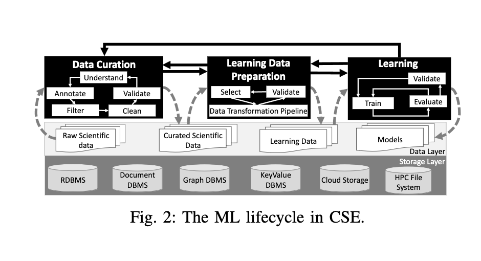
Characterization of Provenance in the ML Lifecycle
Provenance data in workflows contains a structured record of the data derivation paths within a chain of transformations, with parametrization of each transformation. Provenance data are often represented as a directed graph, where vertices represent instances of entities, activities or agents (data, data transformations or users) and edges represent the relationships between them.
A taxonomy is proposed to classify provenance analysis in support of ML:
###### Data Which includes:
- Domain-specific: are the main data processed in the data curation phase. For raw data extraction, quantities of interest are extracted from large raw data files, and for for domain databases, relevant information and metadata are stored in knowledge graphs.
- Machine learning: includes training data and generated training models. Parametrization and data transformation operations are important for provenacen tracking in this category.
- Execution: besides model performance metrics, users need to assess execution time and resource consumption of their workflow. Users need to inspect if a certain block in the workflow is consuming too much resources, or if the execution time is too long. For this, the system is able to capture system perfomance metrics and timestamps.
Execution timing
Refers to whether the execution of the workflow is online or offline.
- Offline: the workflow is executed and the provenance data is captured after the workflow has finished. This is used to support reproducibility and historical results understaning.
- Online: the workflow is executed in real-time, and the provenance data is captured in real-time. The user can inspect the provenance data while the workflow is running. The problem with this mode is that it tends to add high provenance capturing overhead.
Training timing
Refers to the analysis of performance intra-training to inspect one training process, or inter-training to compare different training processes.
- Intra-training: users are interested in understanding how trained models generated in a given context perform.
- Inter-training: users are interested understanding how different training processes compare, which datasets were used, which hyperparameters were used, etc...
ML Provenance Data Representation
The PROV-ML model is proposed to capture the provenance of data in the ML lifecycle. It is built on top of the W3C PROV standard. It inherits the benefits of ProvLake, enabling the integration of provenance of domain specific data processed by ML workflows in the data curation phase.
ProvLake has been applied to capture provenance from multiple distributed workflows that consume that consume and generate data from and to heterogeneous data stores, while keeping the overhead low.
The architecture is build with five main components:
- ProvLake Library: a library that provides a set of APIs to capture and query provenance data. (PLLib)
- ProvTracker: a set of agents that capture provenance data from the execution of workflows.
- ProvManager: a set of agents that manage the provenance data captured by ProvTracker.
- PolyProvQueryEngine: a query engine that provides a set of APIs to query provenance data.
- Prov DBMS: a database management system that stores the provenance data captured by ProvTracker.
The workflows are instrumented with PLLib to capture provenance data. Users can add provenance data capture calls and a data capture task is run when a data trasnformation operation is executed. PLLib tries to keep execution overhead low while avoiding major modifications to the workflow scripts, all the while preserving the provenance data analytical capabilities.
Provenance capture requests are queued and the maximum queue size is a configurable parameter. Moreover, users may chooose to store provenance information on disk only, rather than sending it to ProvTracker.
ProvTracker uses prospective provenance data to provide for the tracking by creating the relationship of retrospective provenance data, being continuously sent by PLLib from multiple distributed workflows. It gives unique identifiers to every data value captured by the PLLib. ProvTracker has several work queues to group provenance requests before sending them to the ProvManager.
ProvManager is a RESTful service that receives provenance data using ProvML vocabulary and transforms the data into RDF triples.
Provenance queries are are provided by the PolyProvQueryEngine.
Execution Strategies on HPC Clusters
ProvLake uses a microservice architecture to achieve high flexibility when specifying how components are deployed to reduce performance penalties.
PLLib is the only component in direct contact with the user workflow running on the cluster. To reduce communication cost between the user's workflow and PLLib, ProvTracker is deployed inside the cluster, on a seperate node.
Provenance Supporting Hyperparameter Analysis in DNNs
Paper | No Code?
The lifecycle of a neural network depends on data configuration decisions that leads to obtaining a succesful model.
Provenance can help in finding the correct configuration for a neural network.

How to capture provenance?
- DNN prov
- Keras prov
Both methods extend from DfAnalyzer, which is a provenance capturing tool for dataflow analysis. Both use the W3C PROV standard for provenance representation.
For DNN prov, the provenance is captured at the level of the model, the layer, the tensor, the operation and the optimizer. The user chooses which data to capture, and has to define the data flow structure in the DNN workflow source code.
These work across three layers:
- Training: library executes model and interacts with Provenance Extractor.
- Data: the Provenance Extractor gets the files (json) containing the DNN information which is relevant.
- Analysis: the Provenance Viewer generates visual representation by querying the provenance database.
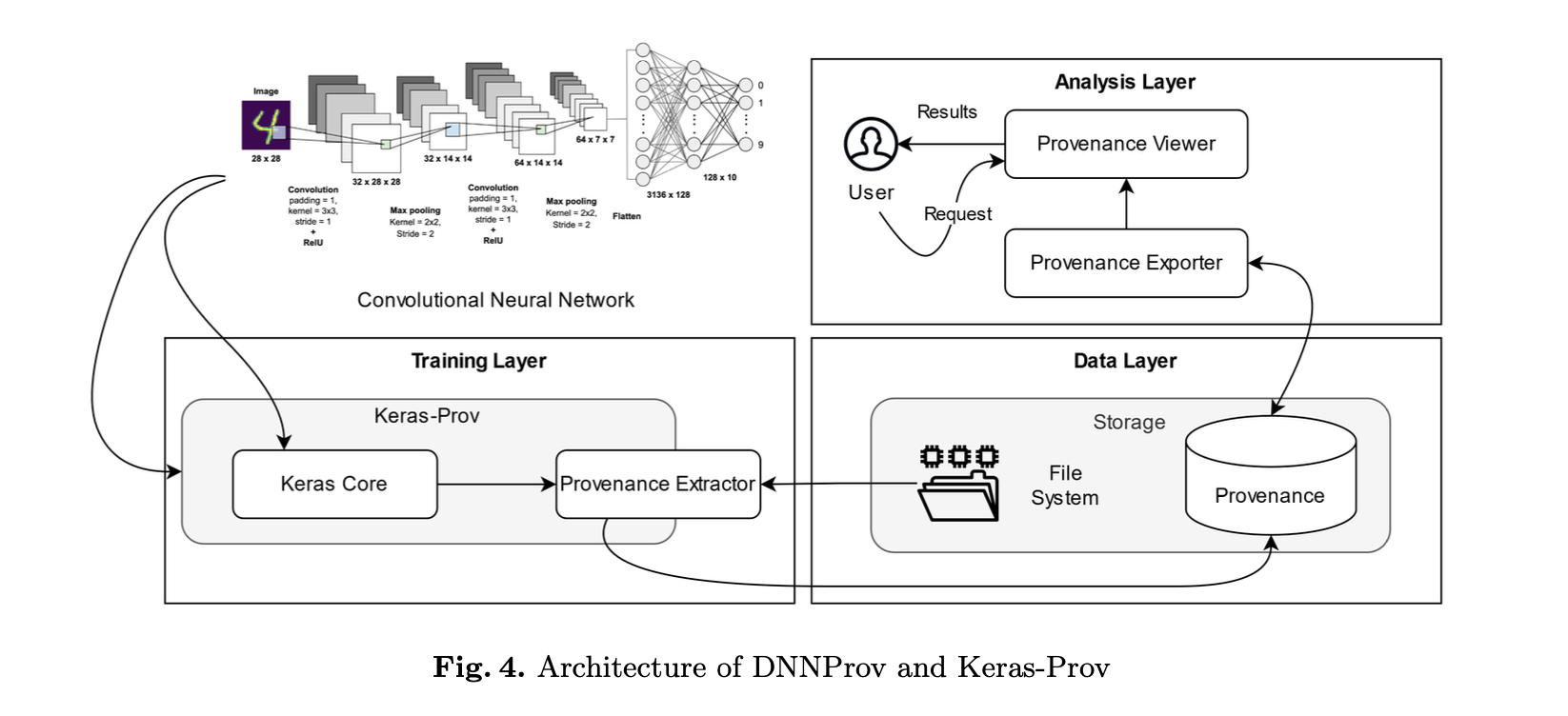
Perpenti Dell'Anna Sengendo Vincze Padovani Atanasova
Data Provenance in Distributed Machine Learning
Paper | No Code?
Data Delineation: crucial aspect of distributed machine learning.
Data Lineage: considers what data is missing, who uses it and what happens (is it modified, updated...).
The pipeline monitors user input, collects information and handles data storage. The pipeline uses UDF (user defined functions) to process data. These are a set of steps of data processing (both intermediate and final data). Generates event logs to the pipeline, then data is stored dumped.
- PM collects information from the pipeline and stores it in a database.
- PM assigns an unique identifier to each data item and evaluates the data and processing.
- Data service handles the storing of data and the processing of data.
- Elastic search gets data from logs and historical data.
- Trustworthyness of data is evaluated by the PM.
- DML is based on SparkSQL and keeps track of the data lineage and records the data logs.
- PySpark is modified to increase accuracy.
To train the model, Stellargraph is used: reads the generated data logs from RDD and PySpark. (and gives resulting logs)
This work tests the trustworthiness of pipeline before training the model.
Keeps overhead under 20% and is able to handle 1000s of data logs. But is higher on compelx queries.
Uses ElasticSearch (paid product) and is not open source. Stellargraph is free and open source, but is not the main focus of the paper and needs provenance retrieval. Competitors are Akka (I think?) and Orleans (couldn't find anything online) (less support for data recovery).
This tool also has no code available I could find...
Linking PROV and XAI in distributed ML
Introduction
The process to register data provenance to guarantee explainability needs to also encompass all pre-processing steps and analyis in the pipeline (not just the ML part). This highlights the need for an end-to-end pipeline for XAI. This also has to take into account data lineage and how and why it got to the present place.
Challenges
To track reproducibility:
- Note the hyperparameters;
- Fix the random interactions and numbers;
- Save all configurations.
Several challenges still persist:
- Make all steps reproducible: which involves making all provenance information available as well as all data processing steps. This involves an active partecipation from both database and ML communities.
- Provenance granularity: coarse granularity is a simple high level description of basic data preparation. Fine-grained granularity implies on the other hand to track all information at each individual record. In many cases, tuple level granularity is enough (adaptable to the ML task at hand, not all projects require the same explainability level).
- Data volume: the solution has to be scalable and we need to store information about which process and node did what. For this, a specialized data format can be used (ex. HDF5).
- Biases and Fairness: biases are accentuated in a distributed environment, where we optimize for speed.
- Data freshness: we should track the time of creation and modification of the ML system and data relative to it.
- Variability and lack of standards: it is not clear which provenance information is needed for an arbitrary ML system. Different communitied need to agree on standards, so APIs for multiple backends, distributed query engines, and data integration systems.
- Data protection and privacy: problem with storing and utilization of sensitive data. Once anonymized, it loses a lot of quality. We need provacy compliant trade-offs, to also provide provenance and XAI. K-anonimity and separation of duties must be expanded appropriately.
IS THERE A WAY TO UNDERSTAND AUTOMATICALLY THE GRANULARITY NEEDED?
Related Stuff
- Provenance for decisionmaking: track data flow to enable identification of entities responsible for actions and decisions (accountability).
- Provenance in a distributed setting: RAMP framework (for map-reduced operator), already implemented in Apache spark.
- Bias: problems related to data (duh), no real solution but mitigation and XAI.
MLFlow2PROV
Introduction
MLFlow allows to simplify the structured collection of artifacts and metadata from ML training. One of its problems is taht is suffers from limited provenance collection capabilities.
MLFlow2PROV is a tool that allows to collect provenance from MLFlow and store it in a PROV-JSON file. Its creates a W3C compliant model which captures ML experiments and and activities from MLflow or other processes. It extracts the provenance metadata grapth from the model, enabling querying, analysis and processing of the information.
It introduces a PROV compliant provenance model (git + MLflow), extracting given a version control repository the provenance of the code and the data. The goal is to capture git related activities (and workflows) and MLflow related activities (and workflows) and to store them in a PROV-JSON file.
PROV recap
-
Agent: An entity that bears some form of responsibility for an activity taking place, for the existence of an entity, or for another agent's activity.
-
Entity: A physical, digital, conceptual, or other kind of thing with some fixed aspects; entities may be real or imaginary.
An entity can beAttributedTo an agent, wasDerivedFrom another entity, wasGeneratedBy an activity, wasInfluencedBy another entity, and wasInformedBy another activity.
- Activity: Something that occurs over a period of time and acts upon or with entities; it may include consuming, processing, transforming, modifying, relocating, using, or generating entities.
An activity can wasAssociatedWith an agent, used an entity, wasInformedBy another activity, and wasStartedBy and wasEndedBy an entity.
MLFlow2PROV Actions
- extract: from the resources of an MLflow experiment, it extracts the provenance metadata graph and stores it in a PROV-JSON file.
- load: file containing a provenance graph
- save: file containing a provenance graph
- merge: multiple provenance graphs into a common graph
- transform: can merge duplicate agents, eliminate duplicate entities, replace user-related info, and so on...
- statistics: print stats for the provenance graph
Process steps:
- input data through for example a yaml file.
- extract provenance VCS repo (git) --> intermediate representation
- extract provenance MLflow and artifacts --> intermediate representation
- provenance graphs generation and processing
- output: provenance graph in PROV-JSON format or document
LIMA: Fine-grained Lineage Tracing and Reuse in Machine Learning Systems
Paper | No code?
Introduction
Data scientists pose hypotheses, design experiments, and analyze results to build machine learning models. This requires building ML pipelines for data cleaning, feature engineering, model selection, and hyperparameter tuning. This causes high computational redundancy which has been adressed in a coarse way.
LIMA offers a fine-grained lineage tracing and reuse system for ML pipelines with low overhead. It captures the lineage of data and models at the level of individual data samples and model parameters. It shows performance improvements of up to 12%.
Data Provenance in ML Systems:
captures information about the origin, processing, and usage of data. Similarly, lineage has been used for low-overhead fault tolerance in data parallel frameworks.
Non-Determinism:
same runs with the same input do not yield the same result. When computing lineage of high level primitives, seed parameters need to be kept into consideration to maintain reproducibility. This non-determininsm limits the use of coarse-grained lineage systems.
LIMA
Uses fine-grained lineage tracing and reuse inside ML systems. A lineage DAG is maintained, where nodes represent the executed operations (including parameters that make them deterministic) and edges are data dependencies. The DAG is recursively built while executing the conditional control flow and operations.
Redundancy
Types of redundancy in fine-grained lineage systems:
- Full function or block redundancy: potential for full reuse of the outputs of a function or block.
- Full operation redundancy: last level operations can be reused for equivalent inputs, given that all non-determinism is exposed to these operations and cast to a basic input as well.
- Partial operation redundancy: operation inputs with oberlappin rows or columns further allow reuse by extraction from (or augmentation of) previously computed results.
These types of redundancy motivate the design with:
- fine-grained lineage tracing and reuse
- multi-level lineage reuse
- exploitation of both full and partial reuse
Lineage Tracing
we introduce the idea of lineage deduplication for loops and functions.
LIMA maintains in a thread lineage DAGs for all live variables of this execution context
A lineage DAG L is a directed, acyclic graph, whose nodes (or lineage items) represent operations and their outputs, and whose edges represent data dependencies. Lineage items consist of an ID, an opcode, and more. Leaf nodes are literals or matrix creation operations (e.g., read or rand), and multiple inner nodes might refer to the same inputs. Thus, the lineage DAG is a data flow graph.
Lineage Tracing:
The immutable lineage DAG for live variables is then incrementally built by lineage tracing as we execute runtime instructions.
Comparisons:
When working with multiple, potentially overlapping lineage DAGs, a key operation is the comparison of two lineage DAGs for equivalence or containment.
Lineage Deduplication:
the problem with fine-grained lineage tracing is that it can lead to very large lineage DAGs. This is due to the repetition of execution paths in loops and functions. This approach uses deduplication as a form of compression, by extracting lineage sub-graphs and storing them only once (as a single lineage item).
- Loop Deduplication setup and tracing: analyze the control flow to aid deduplication. Trace a temporary lineage DAG for each iteration of the loop. Keep a bitvector containing the taken paths.
- Function Deduplication: same process, but for functions without loops or other function calls;
- Handling non-determinism: model the seeds as input placeholders of the lineage path. Trace the seeds and add them as input to the deduplicated lineage DAG.
Also supports task parallel loops.
Experiments
Testing run on
- Autoencoder
- PCA and Cross Validation
- PCA and Naive Bayes
SystemDS with LIMA shows competitive results, even when keeping into account the different level of granulaity of the lineage DAGs this approach is able to capture.
ProvLake
Introduction
Contributions:
- Characterization of the lifecycle and taxonomy of data lineage
- Design decisions to build tools
- Lessons learnt after evaluating on ML application
Captures the entire lifecycle of ML tools, various phases:
- Data curation
- Learning data preparation
- Training
- Evaluation
The paper addresses the challenge of high eterogeneity of different contexts, tools, and data sources. Need to track / assess / understand / explain data, models, and transformation processes.
Creates a comprehensive characterization of the lifecycle of data lineage, and a taxonomy of data lineage (prov to support the lifecycle). Data design to query the provenance data. Creation of Prov-ML (new prov standard) and expansion.
Also set of experiments to showcase ProvML.
Lifecycle of ML Data Lineage
Actors:
- Domain scientists: data curation
- ML engineers: ML model design
(it's a slider, not a binary)
Process includes:
- Raw data
- Data curation
- Domain data
- Learning data preparation
- Learning data
- Training
- Evaluation
- Final model
Provenance data is captured at each stage.
- Domain specific: curation, data and metadata
- Machine learning: data preparation, training, evaluation
- Execution: runtime provenance (info about environment, nodes, etc.)
Types of analysis:
- Online analysis: monitor / debug / inspect in real time
- Offline analysis: post-mortem analysis
Provenance in ML Lifecycle
- Data integration with context aware Knowlwedge Graphs
- Multiple workflows on data lakes
- Keep prospections and retrospective analysis
- Design a conceptual data scheme to capture provenance data
- Easy data linkage and query
Efficient Runtime Capture of Multi-Workflow Data Provenance
PrIU: A Provenance-Based Approach for Incrementally Updating Regression Models
Paper | No code
Introduction
PrIU is a provenance-based approach for incrementally updating regression models.
Incremental view update: iterative process of obtaining the best model for a given dataset, by training over and over removing small subsets.
This paper proposes an efficient provenance-based approach to incrementally update model parameters without sacrificing accuracy (speedup of the train process). Enables provenance tracking and separates the contribution of each sample from the contribution of the model parameters (we can delete the training sample's effect).
This is a framework for provenance tracking and how this can be used for fast model updates. The paper also proposes algorithms for fast model updates when removing a small subset of the training data.
It also enables work on explainability and interpretability of AI models when removing data.
Provenance-Based Incremental Update
How to handle provenance matrices?
- annotate input data with a set of provenance tokens
- propagate tokens through a set of operators:
- + which indicates an alternative
- . which indicates a join
- the application of these operations create provenance polynomials
TODO: continue reading from here
Establishing Data Provenance for Responsible Artificial Intelligence Systems
We first review biases stemming from the data’s origins and pre-processing. We then discuss the current state of practice, the challenges it presents, and corresponding recommendations to address them. highlighting how our recommendations can help establish data provenance
How does data provenance affect the four interrelated characteristics of responsible AI: fairness, accountability, transparency, and explainability?
SOURCES OF DATA BIASES
- Biases from the Data’s Origins
- Population data: developers often rely on access to unique data
- Measurement error: the uncertainty of the input variables resulting either from the measurement itself or from pre-processing is often neglected (the precision of an AI-based system might be overestimated)
- Data quality chasm: lack of data with adequate quality in settings where the AI system is used
- Data repurposing: data collection practices also introduce misuse and biases (repurposing data is the norm in AI-based systems)
- Data augmentation: can amplify existing biases within the dataset and mask the inadequacies of the collected data
- Biases from Data Pre-Processing
- Dataset shifts: non-stationary nature of the environment and the population from which all the input data of AI-based systems are generated
- Opaque pre-processing: in algorithms with intrinsic obscurity, such as deep neural networks, understanding the specific patterns being learned is difficult
- Data labeling: identification and development of labels are often not transparent
- Adversarial manipulation: small changes in the data input can lead to significant differences in the output (susceptible to adversarial manipulation)
- Transfer learning: use the algorithm to solve similar problems
RECOMMENDATIONS FOR IMPLEMENTING DATA PROVENANCE
- Establishing Organizational Data Governance
- Managing meta-data: detailed information about the data captured in a data source (cataloging data and curating data)
- Conducting data audits: assessing whether the data are fit for a specific purpose
- Demanding Data Traceability
- Guiding data acquisition: Manual labeling regulation
- Benefitting from blockchain technology: potential to upgrade the value of the data and provide more efficient and transparent results
- Leveraging Technological Advances for Data Provenance
- Deriving explanations: XAI methods, such as LIME, LORE
- Managing noisy data: attributed noise from features or class noise from labels/targets
- Identifying inherent data structures: clearer understanding of the system’s behavior and the data helps judge the fair- ness of recommendations
Provenance documentation for XAI
Provenance documentation is one of the means to accomplish transparency, traceability, explainability, and reproducibility in AI-based systems.
Inter-relationships between XAI, TAI, and provenance through a bibliometric analysis.
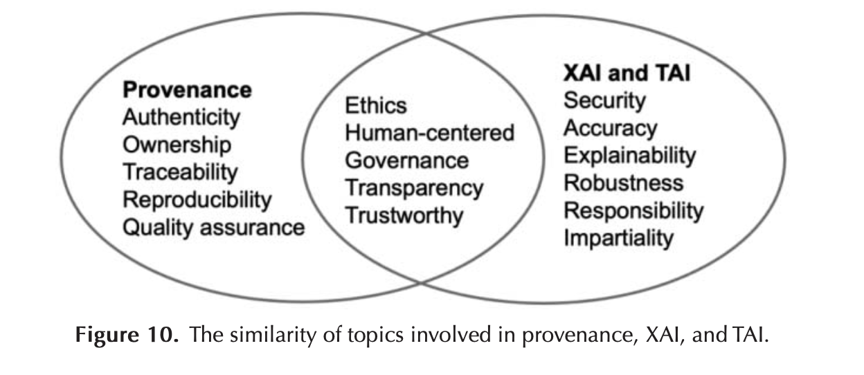
Data Provenance Initiative
The Data Provenance Initiative’s goal is to audit popular and widely used datasets with large-scale Legal and AI expert-guided annotation.
Development of a set of indicators necessary for tracing dataset lineage and understanding dataset risks.
The initiative’s initial focus on alignment finetuning datasets was decided based on their growing emphasis in the community for improving helpfulness, reducing harmfulness, and orienting models to human values.
The DPCollection annotation pipeline uses human and human-assisted procedures to annotate dataset Identifiers , Characteristics , and Provenance.
Data Provenance Explorer (DPExplorer)
"We release our extensive audit, as two tools: a data explorer interface, the Data Provenance Explorer (DPExplorer) for widespread use, and an accompanying repository for practitioners to download the data"
Collecting comprehensive metadata for each dataset required leveraging several sources including collection by linking to resources already on the web (e.g., dataset websites, papers, and GitHub repositories).
License Annotation Process
One of our central contributions is to validate the licenses associated with widely used and adopted datasets.
Research Object Crate (RO-Crate)
Workflow Run ROC
The problematic part of scientific recording is the provenance of its outputs.
ROCrate
Packages research data with metadata from platform
Workflow Run ROC
Represents computational workflow execution provenance (both prospective and retrospective).
IMP: look at SKOS and AUTOSUBMIT
3 profiles:
- Process Run Crate: execution of one or more tools
- Workflow Run Crate: execution of predefined workflow
- Provenance Run Crate: collects internal details of each step
Problem: during development, developers don't like to handle wfs. But that's where the important provenace is collected.
Collecting, Managing, and Analyzing Provenance Data
Taxonomy of provenance from scripts --> collection + management + analysis
Tools for collecting provenance data from binaries execution, collect info about OS, hardware, syscalls, etc. Each provenance type refers to a different collection technique / mechanism.
Annotation: either on procedures or on data. Identifies through placement, target, inclusiveness, extraction, and necessity.
Provenance based IDs
Not yet mature. Robustness against dedicated adversaries is not yet proven.
It offers:
- Runtime behaviour training
- Finetune ML systemon prov files
- Unified event format
Adversarial validation is necessary to prove robustness. Problem space is critical, requires knowledge of the system (domain knowledge).
Data guided attach search through ProvNinja.
- Identifies conspicuous events (data + attack graph)
- Replace with common events (search for replacement with attack grapth and event summary)
- Camouflage process: summarize the expected behaviour (execution profile + expected behaviour). Mimic benign behaviour from an incouspicuous attack grapth (camouflaged).
- Validate: feature space validation, problem space validation, implementation, integration, and deployment.
This method decreases detection rate of attacks by 57%. Supports adversarial testing and verification.
LLM Carbon
High-Velocity AI Cache (HVAC)
Distributed deep learning training time can be divided into three parts:
- computation time
- communication time
- I/O time (67% - 85% of the total time)
It's a caching library for AI applications. Uses node-local storage on compute nodes + near node-local storage on the network for caching on the parallel filesystem. Distributed hashing is used to determine the cache location.
All items during training are traversed one time for each epoch. Between epochs items are shuffled.
- Within the DL job we have high shareability of I/O (several passes over the same data (cache friendly)).
- Random access pattern for each epoch is bad.
- The random sequence order is not correlated with accuracy, therefore I/O is substitutable.
HVAC uses a client-server architecture.
- The server uses node-local storage across the compute nodes, spawns a dedicated data mover thread managing a shared FIFO queue for I/O requests (aggregated shared cache layer on node local storage).
- The client intercepts I/O calls and registers and sends them to the server.
Computational and Energy Use of CMIP6
Design of CPMIP: computational performance CMIP6, designed to assess model performance and cost of running these simulations.
Result: ~1600T of CO2Eq
Total energy = Simulated years x JPSY (Jouls per simulated year)
Carbon footprint = Total energy x CF x PUE
where:
- CF = Greenhouse gas conversion factor (MWh to CO2Eq)
- PUE = Power usage effectiveness (accounts for data center effectiveness)
Useful metrics:
- SYPD: simulation years per day
- CHSY: core hours per simulated year
- Parallelization, complexity, and resolution: cluster / experiment dependant metrics (constant values)
- Data output cost: greatly influenced by I/O configuration
- Data intensity: production efficiency of data (data generated per core hour, correlated with SYPD)
- Workflow and infrastructure cost: cost of running the simulation, very much infrastructure dependant (11% - 75% of total cost)
- Coupling cost: cost of coupling ESM models
\( CC = \frac{T_M P_M - \sum_c T_C P_C}{T_M P_M} \)
where:
- \( T_M \) = total runtime for model
- \( P_M \) = parallelization for coupled model
- \( T_C \) = total runtime for individual component
- \( P_C \) = parallelization for individual component
Other metrics:
- Speed / cost / parallel: closely related to model speed and parallelizability
- Memory bloat = (Mem size - Parallel x File size) / Ideal mem size = ~ 10 - 100
- Useful simulated years: years that are actually used for analysis
- Data produced: data generated by the simulation
How to estimate missing numbers? mean(ESGF data) or mean(Total data) or mean(ESGF data)
Energy intensity of internet data transmission
Estimation of how much energy is necessary to transmit data over the internet (KWh / Gb).
New criteria is given, plus new estimate for 2015 of 0.06 KWh / Gb. This results in 50% less cost since 2000, which is comparable to the energy and performance increase in computing.
- Bottom-up approach: sum of all electricity consumption / data transmitted through equipment (underestimation)
- Top-down approach: network electricity used / total data transmitted (overestimation)
New method is weighted average of previous estimations + regression on historical data for validation.
Subdivision is different groups of consumption: data centers; undersea cables; IP, access, home networks; and end-user devices.
Green AI
Comparison of ML frameworks in terms of energy efficiency, carbon emissions, and computational cost.
Three frameworks are compared: TensorFlow, PyTorch, and MXNet.
Environment chosen is using Nvidia RTX 3070 with 8 Gb of memory, energy data is collected sampling from nvidia smi.
- How do they differ in terms of energy efficiency?
Recording of GPU power / utilization / energy + partitioning for each HW component.
Torch is better with larger batch size and with larger models (prob. due to better parallelization) (ex. BERT).
MxNet is better with batch size of 1.
- How do execution providers differ in terms of energy efficiency or performance?
Comparison between CUDA / Tensor RT
Tensor RT always outperforms CUDA, why? It utilizes GPU more effectively (> GPU utilization).
Green 500 Metrics
- GFlops/Watt: the number of floating-point operations per second that can be executed by a computer, divided by the power consumed by that computer
- Power (kW): the power consumed by the system
- RMax (PFlops/s): the maximum performance of the system (practically achieved)
- RPeak (PFlops/s): the theoretical peak performance of the system
Utils
The heat dissipation is a problem with large clusters, this means that the delta between the power consumed and the power dissipated is not negligible (RMax - RPeak). This is a problem because the power consumed is the power that the system is drawing from the grid, and the power dissipated is the power that the system is actually using. This means that the system is not using all the power that it is drawing from the grid, and this is a waste of energy.
Green Destiny: low power supercomputer, no unscheduled downtimes despite no cooling, humidification or air filtration.
Green500: treats both the power consumed and the performance
- SPEChpc.
- ED^n metric: Energy Delay product, the product of the energy consumed and the time taken to complete a task.
- FLOPS/Watt: the number of floating-point operations per second that can be executed by a computer, divided by the power consumed by that computer. (Might be biased towards small supercomputers, so measure one node only and then multiply by the number of nodes)
Making the case for Green 500 List
- ED or ED^2 or ED^3: Energy Delay product, the product of the energy consumed and the time taken to complete a task.
- V_0 = E^(1-theta) * D^(1+theta) where theta is a parameter that can be adjusted to reflect the importance of energy and delay in the metric.
Escapedes to Exascale
GreenIndex (TGI): measures the efficiency with regards to a reference system. Where i indicates a specific benchmark.
- EE_i = Performance_i / Power_i
- Relative EE_i = EE_i / EE_ref
- TGI = sum_i (W_i * Relative EE_i)
Data centers energy efficiency
For power and energy efficiency
Holistic power management:
- Resource provisioning and stranded power (this includes power and cooling, it's around 50% of all power).
- Reduce perfoemance but but increase energy efficiency.
- Increase / reduce speed selectively at runtime (not before the scheduling). It automatically estimates the type of compute/memory bound process.
- Performance to sustainability slider.
LSTM Vis
Understand RNN through visualization. Three types of users:
- Architect: new deep learning methodologies
- Trainers: apply architectures to domain
- End users: use general purpose pretrained models (XAI)
Use cases:
- Generate an hypothesis about properties of hidden states
- Refine hypothesis
- Compare models and datasets
- Visualize hidden states / filter hidden states
- Match selections to similar examples
- Align textual annotations + interface
This tool also gives per-token insight into the hidden states of the model.
Relationship between H-state and Semantic Structure
Research questions:
- Are the hidden states linearly separable?
To gain insights into the structure of hidden states (linear separability is a requirement for clustering)
- Is the clustering hypothesis valid?
Definition of a cluster and usefulness of a cluster, Do hidden state cluster correlate with DFA?
Results shown are "often linearly separable", not quantifiable.
Also very formal language paper (not quantifiable).
Hidden Memories of RNNs
Understanding RNNs: lack of interpretable models, hidden states, and the role of memory.
- Performance based: alter the components and see how it affects the accuracy.
- Interpretability extension: visualization (and comparative clustering), use adjacency metrics.
- Justaposition: detail / sentence / overview level
- Superposition:
- Explicit encoding
Requirements
-
Interpret information captured by hidden states / layers
-
Provide information distribution
-
Explore hidden states at sentence level
-
Examine stats for hidden states
-
See learning outcomes
-
See distribution of hidden states
-
See model expected response based on update of cell
-
C = maintains long term memory
-
h = directly computed from cell state and used for output
-
Dc = distribution of cell states change
Co cluster hidden states and words to see how they are related. Also sequence analysis to see how hidden states change over time.
Analysis of Entropy in Hidden States of RNNs
Entropy lowers similarly to the training loss?
What does it mean if the entropy lowers?
- In hidden states: means that the process is becoming more predictable. (overfit?) (vanishing gradients?)
- In general: less entropy means that items of the tensor are more and more similar to each other.
We don't want entropy to drop too much in the training process.
TODO What happens if we overfit the model (smaller hidden size)?
Notes on Talks
A Data-Oriented Perspective
These are Data-Driven approaches
Here are the major climate-centered datasets used in the field:
| Dataset | Size | Where? |
|---|---|---|
| MACCA | 60 TB | Nasa |
| CMIP6 | 25 TB | |
| Earth System Configuration Grid | 25 TB | ORNL |
| ERA5 | 1.5 PB | ECMWF |
| ARM | 50 TB | ORNL |
Information as value chain: how information is created, stored, and used in a particular context.
- How can we do this?
- How are agencies taken from agencies and used in the field?
- Is data free of errors?
- Without any bias?
- Is the data reliable?
Model Summary
Here are some of the state-of-the-art models in the field and their performance:
| Model | Precision | Forecast time |
|---|---|---|
| PanguWeather | < 50 m | 7 days |
| GraphWeather | < 50 m | 7 days |
| GraphCast | < 60 m | 8 days |
| ClimaX | < 100 m | 7 days |
Other approaches:
- Swin-SpatioTemporal Transformer: currently evaluated for NASA project Higher complexity, better for small scale
- Spherical Fourier Neural Transformer: to avoid noise and blurring problem Due to spherical projection of grid, problem is accentuated at the poles. This model is able to avoid this problem, using this operator for sphere geometry.
- GraphCast is better at small resolution and at different scales. Also better at compressing information.
- IFS uses global 9 km resolution data. On long term forecasts, it is better than ML models. However with higher resolution data (25km data), ML models are better.
- Ensamble Forecasts: run several simulation from same initial conditions, and average the results. This is a common technique in NWP. Same approach can be used for ML models.
AI 4 Good
Second Climate Forecast Revolution
As the first one revolved around Numerical Weather prediction forecasts (solving physics equations to predict weather eg. IFS).
Weatherbench 1
First attempt at a ML data oriented approach to weather forecasting. First winter of AI for climate, as not enough data was available. Data-based approaches were not precise enough to reach NWP levels of accuracy.
Weatherbench 2
- Data: in Zarr format + IFS baselines
- Evaluation Code: usind datacloud or other remote computing services (colab, aws, etc)
- Evaluation platform: interactive graphs, for user visualization
Are AI models just blurring?
How do we understand this factor? First we can check if the model is able to predict extremes (or is just averaging the data).
Blurring exists, but is limited to small scales and does not influence the prediction of extremes. Many ML models have been used for Hurrican Season prediction. Graphcast is better than NWP.
Tropical Cyclones
Quick Notes
Structure: cyclones develop in the presence of these conditions:
- warm water of tropical oceans (>26.5C) → collects energy through convection (?)
- unstable atmosphere, cooling fast enough to cause thunderstorms
- moist middle atmosphere (humidity)
- low vertical wind shears, and little change in wind direction with change in height
Tropical Cyclone Genesis potential index (GPI) → accurate, but only at low resolutions
Often these are good for spatial correlation but bad for temporal one (difficulty in predicting inter-annual events) Solution is to use evolutionary algorithms to obtain Pareto Front of possible solutions (all possible optimal trade-offs between spatial and temporal optimality) → all solutions still have non acceptable temporal resolution.
Tropical storms are very rare, lots of samples where the event returns negative, only a small portion positive.
Physics
A tropical cyclone is a storm system that rotates rapidly, featuring a low-pressure center, intense winds, and an organized series of thunderstorms that cause intense rain and sudden gusts. The term tropical refers to the geographical origin of these systems, which form almost exclusively over tropical seas, while cyclone refers to their winds moving in a circle, around a central eye, with surface winds blowing counterclockwise in the Northern Hemisphere and clockwise in the Southern one. These cyclones have a diameter most often found between 100 and 2,000 km. The powerful swirling winds of a tropical cyclone, as the ones shown in Figure 2.3, arise due to the Earth’s rotation imparting angular momentum as air moves towards the axis of rotation. These storms are generally most severe when over or near water and quickly lose intensity when moving over land. Damage can result from strong winds, rain, high waves, and storm surges, all of which are phenomena of rising water caused by high-speed winds pushing water towards the coast.
These tropical storms are low-pressure regions in the troposphere. The pressure is the lowest near the surface, while at the center of these storms sea level pressures are among the lowest ever observed. These systems are called ”warm core” because the environment near their center is warmer than the ambient temperature at all heights. At the periphery of the storm, the air may be nearly calm; however, because of the Earth’s rotation, the air possesses non-zero absolute angular momentum. As the air flows radially inwards, it starts rotating cyclonically so as to conserve angular momentum effectively. At a certain distance from the centre of the storm, air starts moving upwards towards the top of the troposphere. The air, once lifted, moves away from the storm’s centre and forms a layer of high clouds called ”cirrus clouds”. These processes ultimately create a wind field that is almost symmetrical around the storm’s centre. Wind speeds are low at the centre, increase moving outwards towards the radius of maximum winds and then decay more gradually with radius.
Comparing State-of-the-Art Models
Challenges and Opportunities
Difficulties
- Post-processing of data
- Costs for specific scenarios and analysis (ex. outliers in rare events)
- Under-utilization of existing data since it is expensive to process
- Data quality and quantity
Opportunities
- Multimodal models: radar, satellite, numerical weather prediction, etc.
- Interpretable models / explainable AI / causal AI
- Generizable models
- can the model predict out of scope?
- can the model avoid bias and flaws in the training data?
- Continuous learning: can the model learn from new data?
- On-device adaptation: customize a model based on local data (ex. adjust to local climate)
- Federated Learning: each company trains their own model, but they can share their models to improve the overall model. Global model learns from updates from local models.
Foundation Model for Climate Improvements
Incremental Probability in Cyclone Prediction
One possible improvement to the presented work arises from the fact that the dataset currently illustrates the likelihood of a cyclone being present in a patch with a simple Gaussian distribution. Nonetheless, as the weather variables increasingly make it more plausible, the probability of a cyclone should raise over time. It may be possible to encode this behaviour by manipulating the standard deviation parameter of the Gaussian, resulting in the probability area progressively expanding over time. This would require determining when a patch is displaying indications of forming a tropical cyclone and identifying the exact central position in the patch.
Parameter oriented training
One of the main differences between the current implementation of the model and the one presented in the ClimaX paper, is the fact that the latter is trained to predict the input variables shifted by a certain amount of lead time, and the training is repeated for several lead times. This allows the architecture to learn the correct behaviour of each variable over time, and enhances its flexibility by allowing at inference time to take a lead time parameter, and output the correct prediction. This approach has been referenced to as ”parameter oriented training”, and by its very flexible nature allows for a more general purpose model, which can be used for several different tasks.
Global forecasting system
In a similar way to ClimaX’s approach, it may be feasible to merge the image patches and generate a worldwide weather forecast. This would not necessitate any modifications to the current model since the global image normalization is already executed. Additionally, the dataset can be adjusted to share an N-pixel border with adjoining patches and prevent loss of nearby data. This modification addresses weather variable forecasting and has no impact on this project’s fine- tuning section. Predicting global cyclones may not be necessary since the regions where they most often form are widely recognized, and a regional forecasting approach would be enough.
Time-Series Transformers
Among several advantages of the transformer architecture, the ability to capture long-range depen- dencies and interactions is particularly central to time series modeling. A possible improvement to the current work could revolve around increasing the dimensionality of the input data by adding a temporal dimension, and using this information to better predict the future weather. This would imply passing a sequence of time snapshots to the model, and the tensor’s dimensions would become <B, T, V, H, Lat, Lon>, where T is the number of time snapshots.
As for the modifications necessary to the current architecture, the positional encoding of the transformer has to be changed, to allow for the correct encoding of the temporal dimension. What has been done in similar works, is allow for the embedding to be learned from time series data, and not be fixed as in the current work. A similar approach is to use the timestamp information to influence the training of these embedding layers, and allow for a more accurate representation of the data.
Ensemble of models
Connection to the Intertwin project
One possible mean of unifying the two works could revolve around the use of graph neural network architectures, and integrating these mostly novel approaches into large foundation models. While Fronza’s work revolved around graph neural networks, there exist in the literature examples of applications of these kind of models to global weather forecasting, which is an essential requirement for developing a foundation model based on GNNs. These techniques have already been tested in the literature, where Graph Transformers are used to generate text, processing both the data with the classical approach, but also building a knowledge graph of the sentence, enhancing the understanding of the context. This approach could be used to build a foundation model which is able to understand the context of the input data, and use this knowledge to improve the prediction ability of the model. In this case, the context could be the current regional weather, and the model could use this information to better predict the future weather
Weights and Biases Webinar
- Sweep Feature: log hyperparameters optimization (e.g., learning rate, batch size, etc.)
- Frozen run: interrupt and continue training (freeze configuration values)
- If GIT: check if a change is unstaged and take note in a diff file. Also check modifications in a notebook, if one is being used.
- Differences tables to check differences between runs (this is done in the explorer a posteriori)
- Tracking of system metrics both at process and system level (tracked every 20 seconds, so running averageis visualized)
- Lineage Tab: track different versions of the pipeline. Create / Consume artifacts (ex. create artifact of dataset for train / test split)
- Artifacts tab: log any file with run checksum (optmized for large files, so you don't have to store multiple copies of the same file)
- Register model to link to similar versions
ZERO
Eliminates memory redundancy (model state is the source of largest memory usage).
- Data Parallelism: poor memory efficiency
- Memory Parallelism: poor compute efficiency and communication overhead
Zero DP: data parallel efficiency + efficient communication
- Optimizer state partitioning: 4x memory reduction
- Gradient partitioning: 8x memory reduction
- Parameter partitioning: memory reduction proportional to the number of partitions (DP degree) but 50% more communication volume
What is left is residual buffers / activations / gradients
Zero-R optimizes activations memory
- Identifies activations replications
- Defines optimized state for temporary storage / buffers
- Manages memory based on lifetimes to prevent memory fragmentation
Is ZERO + MP useful? It can reduce memory footprint of very large models.
Zero ++
Improvement on Zero redundancy optimizer.
Cons: when on low bandwidth clusters, or with small batchsizes, the high communication overhead can be a bottleneck and lower the effectuve throughput.
Communication volume reduction techniques:
- Block quantization for allgather: shrink down all model parameters to a single block, block based quantization (indipendent for each set of model parameters);
- Data remapping that trades off more memory for less communication: hierarchical weights partitioning (maintain a copy of the model in each partition, but only update a subset of the weights in each partition);
- All to all quantized gradient averaging paradigms: new gradient communication paradigm that reduces communication volume. Gradient compression with block based INT4 quantization, but the precision is recovered before the reduction operator to preserve the accuracy of the final model.
4x reduction in comms volume, 2x better throughput.
Comms volume reduction: from 3M to 0.75M.
Fire Behavior
Variables
- Ground truths: GeoMAC fire database (ALL WORLD) ()
- Weather data: NOAA (ALL WORLD) ()
- Satellite visual imagery: ASK VAL (BOH) ()
- Digital elevation model: ASK VAL (heightmap) (or also found) (BOH) (cropped)
- Fuel data: CBD landfire data (fuel type) (USA) (cropped)
- Land Cover: C-CAP (type of ground) (USA) (cropped)
Data
Landsat 8
High-resolution land cover data. Resolution: 1 to 2.4 meter, 25 categories
All Downloads are Here
World View 2
How To Access Data --> Project Proposal (Restrained) 2009 - present
Wildfires
Resolution: 1km
GeoMAC
Better res I think
Global Wildfire Information System Initial Spread Index | Global Fire Atlas with Characteristics of Individual Fires, 2003-2016
Fire Fuel
Near real time
LANDFIRE's (LF) Forest Canopy Bulk Density (CBD) describes the density of available canopy fuel in a stand. It is defined as the mass of available canopy fuel per canopy volume unit.
DEM
30m resolution
MODIS
ChatGPT for Global Warming
Climate change requires inter-disciplinary appproach with several topics (atm. science, oceanography, biology, etc.). ChatGPT could help with:
- Data analysis and interpretation
- Communication of complex information wo wide audience
- Decision making and recommendations
- Climate scenario generation, with alternative inputs
Limitations:
- Understanding complex concepts (scientific background, may not understand scientific correlations)
- Lack of contextual awareness
- Biases from training data
- Accountability for decision and output (ethical problems)
- Limited scope of expertise (up to date knowledge problem)
TODO: CAN WE TRAIN IT ON DAILY INFORMATION, TO KEEP IT UP TO DATE?
Machine Learning for Climate Change Research
Climate change research will require high adaptability to understand better the complete climate system.
Problem of uncertainty: more data in some instances could be useful.
Dimensionality reduction: differential equation govern how ESM behave --> complex There are three main approaches:
- non-dimensionalization of equation term: create reduced set of linked equations
- dimensional analysis: both collapse the complexity and relate different strands of data (linkage can aid reconstruction, parametrization or testing)
- statistical techniques: using empirical orthogonal functions (EOFs) to reduce the dimensionality of the data
- emergent constraints (EC): refine projections by searching across ESM ensembles for regression between modelled climate systems
How to integrate ML with these reduction techniques?
Machine Learning applications in climate
- Extreme events forecasting
- Uncertainty in climate response
- Build ecological-climate equations (interactions)
The key interaction equations are known
- Ecosystem photosynthesis, respiration and decomposition
- Operate at individual tree level
- Unknown are the equations that capture complex canopy structure and temperature-dependant variations in leaf processing. It can cause uncertainty in global carbon fluxes.
Incremental Models
Literature Review
Growing LSTMs
Growing LSTMs is a technique used to accelerate the training of deep learning models, particularly LSTMs, by incrementing the size of the model during training. A general heuristic decides when to add a block through two techniques:
- Cascade: weights which come from an existing block are copied to the new block.
- Fully Connected: all hidden weights are modified.
Nest
Gradient based growing:
- connection growth: greedily activates dormant connections (add connection only if the loss is reduced)
- neuron growth: connection estabilishment + weight initialization. Add neuron between Node i and j if correlation pre-synaptic and post-synaptic is high.
Magnitude based pruning: remove connections if magn(W) is less than a threshold T.
Partial Area convolutions: convolve only the area of interest, not the whole image. (CNNs are computationally expensive)
Learn Weights and Connections
Also does pruning, learns which connections are important, then prune weights. Converts dense net into a sparse one.
Grow and Prune LSTMs
Based on the H-LSTM cell (Hidden layer LSTM). The difference comes from the weight update vector, which is replaced by 4 DNNs with multi-layer transformations. This gives more control, easy regularization and flexible gates.
Process:
- initialize the H-LSTM cell with a single layer LSTM
- grow the H-LSTM cell by adding a new layer + training the model
- activation function + more training
- pruning of connections + training
- final model
Layer Stacking
From the observation of layers:
- Attention distribution on shallow layers is more uniform across different positions and layers. Distribution in shallow layers focuses on neighboring tokens + the starting token.
- Attention distribution in deep layers is similar to the distribution of shallow layers (knowledge can be shared).
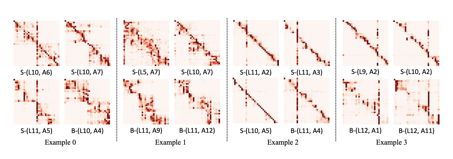
Layer stacking implies copying weights in new layers from the previous layers. This is a way to increase the depth, with an additional warm start. At specific iterations the model doubles in size.
Layer Dropping
Layer dropping accelerates the training of Transformer-based language models. Transformer-based language models have achieved remarkable performance in many NLP domains, but the unsupervised pre-training phase of these models suffers from unbearable overall computational costs. Layer dropping is a method to accelerate the pre-training of these models, not at the cost of excessive hardware resources, but from the enhanced efficiency of modifying the model architecture and training technique.
Layer dropping involves the random removal of layers from a neural network during training. This has the effect of reducing the depth of the network, which can speed up training. However, it has been observed that random removal of Transformer layers destabilises performance and easily results in serious consequences such as model divergence or convergence to an erroneous/suspicious local minimum
RHO
RHO-LOSS (Reducible Holdout Loss Selection) is a technique introduced to accelerate the training of deep learning models by selecting the most useful data points for training. Instead of training the model on all data points uniformly, RHO-LOSS selects the points that are most likely to reduce the generalisation loss of the model.
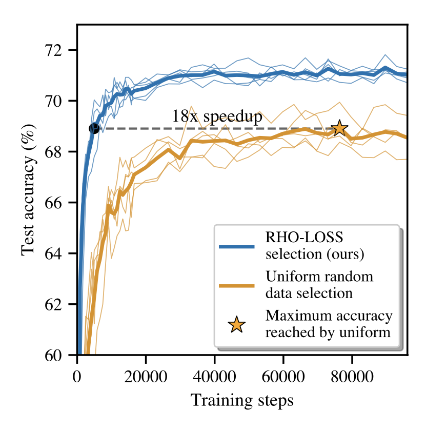
RHO-LOSS offers several advantages, including:
- Accelerated training: it can significantly reduce the number of training steps required to achieve a given accuracy, as demonstrated by experiments on various datasets, including the large dataset of web-scraped Clothing-1M images
- Improved accuracy: in addition to accelerating training, RHO-LOSS can also lead to improved final accuracy of the model
- Robustness: RHO-LOSS has proven effective across a wide range of datasets, hyperparameters and architectures, suggesting its robustness and general applicability
LiGO
LiGO is a technique used to accelerate the training of deep learning models, particularly Transformers, by reusing weights from smaller pre-trained models. The key idea is to map the weights of the pre-trained model to those of the target (larger) model using a linear growth operator that expands the weights of the pre-trained model to those of the target model.
Claims of LiGO:
- FLOPS: -40%
- Wall-clock time: -50%
- Params: ??
Mango Operator
The Multi-linear Operator (MANGO) is a technique used to accelerate the training of deep learning models, particularly Transformers, by reusing weights from smaller pre-trained models. The key idea is to map the weights of the pre-trained model to those of the target (larger) model using a multi-linear operator that captures correlations between all the weights in the model.
Previous methods for reusing pre-trained models, such as bert2BERT and LiGO, focused on mapping only part of the weights, ignoring potential correlations between the entire model. For example, bert2BERT expands the width of the model head by head in Transformers, while LiGO focuses mainly on extending weights of the same type (e.g. query, key and value in Transformers). This partial mapping approach may not be able to capture all useful information from the pre-trained model and lead to sub-optimal training. MANGO addresses this problem by considering the interaction between all model weights. Instead of a partial mapping, MANGO proposes a complete mapping that linearly links each target model weight to all pre-trained model weights. This approach makes full use of the correlations between the weights and results in a more accurate mapping.
The direct use of a full mapping operator would involve a huge parameter tensor, making the process computationally prohibitive. To overcome this obstacle, MANGO uses a multi-linear decomposition, specifically the ring tensor matrix product operator (TR-MPO), to decompose the large mapping tensor into four smaller tensors. This decomposition significantly reduces spatial and computational complexity, making MANGO practical to implement.
The main advantages of MANGO are:
- Faster training speed: MANGO significantly speeds up the training of large models compared to training from scratch or using partial mapping methods.
- Improved accuracy: MANGO can lead to models with better performance than previous methods, as it can better capture correlations between model weights.
- General applicability: MANGO can be applied to different types of Transformer models, as demonstrated by experiments on DeiT, BERT and GPT.
How to apply MANGO?
- Concatenate weights of pretrained model to construct Mi matrix
- Train growth operator ϕ
- Recover weight tensor M2 with multi linear operator
- Split M2 weights
Lion
Selective Backpropagation
Efficient Training for Transformers
Three categories of methods to accelerate training of Transformers:
- Dynamic architectures: layer dropping, layer stacking
- Batch selection: RHO-LOSS, selective backpropagation
- Efficient optimizers: Lion
How to compare training?
- Iterations: BAD, may change time per iteration
- FLOPS: BAD, not taking into account parallelism
- Wall-clock time: BAD, fluctuates even when using the same HW
- Reference time system: GOOD --> how to calculate?
RTS = time_per_iteration_compute * time_per_iteration_on_reference_system
Results:
- Dynamic architectures: no improvement
- Batch selection: no improvement
- Efficient optimizers: no improvement
RNNs Shortcomings
- Are not guided in the compression process of information (there is probably a better way for them to learn important tokens).
- How do we learn the important tokens? We understand the context.
Or maybe we just base importance on the length of the token. How do we know the importance of a token if we encode it in a fixed size vector? Size dependant encoding?
IMP: this doesn't work with images.
Scaling Issues
In this section, we will discuss the scaling issues that arise when training large language models (LLMs) and recurrent neural networks (RNNs). We will also explore some of the solutions that have been proposed to address these challenges.
Transformers
Transformers have become the dominant architecture for natural language processing (NLP) tasks due to their superior performance on a wide range of benchmarks. However, training large transformer models comes with its own set of challenges, including scalability issues related to memory consumption, computational complexity, and training time.
Quadratic Time Complexity in Attention Mechanism
The self-attention mechanism in transformers has a quadratic time complexity of O(n2)O(n2), where nn is the sequence length. This means that the computational cost of processing a sequence grows quadratically with the length of the sequence, making it challenging to scale transformers to handle long sequences.
Scalability Issues
These models require large amounts of memory and computational resources to train effectively. As the size of the model and the dataset increases, the memory requirements and training time also grow significantly. This can make it difficult to train large transformer models on standard hardware or even high-performance computing clusters.
Some Solutions
To address these scalability issues, researchers have proposed several techniques to improve the efficiency of transformers and reduce their memory and computational requirements. Some of these techniques include:
Linformer: This model approximates the self-attention mechanism, reducing the complexity from O(n2)O(n2) to O(n)O(n) in certain scenarios. Longformer: Uses a combination of local and global attention to handle longer sequences more efficiently. Performer: Applies kernel methods to approximate the self-attention mechanism with linear complexity. Reformer: Utilizes locality-sensitive hashing (LSH) to reduce attention computation, achieving sub-quadratic complexity.
RNNs
Recurrent neural networks (RNNs) have been widely used for sequential data processing tasks due to their ability to capture temporal dependencies in data. However, training RNNs on long sequences can be challenging due to issues such as vanishing and exploding gradients, sequential computation, and difficulty in capturing long-term dependencies.
Sequential Computation (Time Complexity)
RNNs process input sequences one step at a time, where each step depends on the previous one. This inherently sequential nature means that the operations for each time step cannot be easily parallelized. As a result, the time complexity of RNNs is O(T)O(T), where TT is the sequence length. This makes RNNs relatively slow when dealing with long sequences, especially on modern hardware like GPUs, which are optimized for parallel computations.
Vanishing and Exploding Gradients
During backpropagation through time (BPTT), which is used to train RNNs, gradients are propagated through many layers (one for each time step). For long sequences, this can lead to vanishing gradients, where the gradients shrink exponentially, making it difficult for the network to learn long-range dependencies. Conversely, gradients can also explode, causing instability and large updates that make the network difficult to train.
Difficulty in Capturing Long-Term Dependencies
RNNs have a limited ability to capture long-term dependencies due to the vanishing gradient problem. This can lead to the loss of information over long sequences, making it challenging for RNNs to model complex relationships in the data effectively. Also, considering the hidden state as a context memory cell, the model has a fixed amount of memory to store information from the past. This can limit the model's ability to capture long-term dependencies effectively, and may lead to information loss over time.
Some Solutions
- Better compress the information in the hidden state.
- Incrementally grow the model's memory capacity as needed.
- Use attention mechanisms to focus on relevant parts of the input sequence.